This blog documents my notes on 16. Learning: Support Vector Machines.
I try to fill the gap in the explanations in Prof Patrick Winston's lecture.
Support Vector Machine problem statement
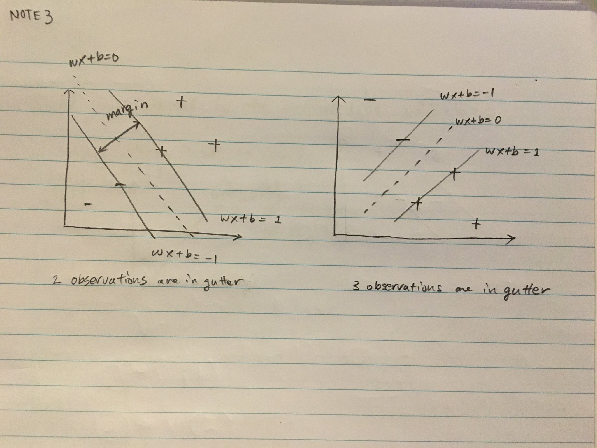
Given two class observations (linearly separable for the sake of problem understanding), find the best line that maximizes the margin (or the distances of the two streets) between + and - observations!

Decision Rule
Some unknown observations $\boldsymbol{u}$, we classify them as $$ \boldsymbol{w}\boldsymbol{u} + b \ge 0 \rightarrow \textrm{classified into +}\\ \boldsymbol{w}\boldsymbol{u} + b < 0 \rightarrow \textrm{classified into -}\\ $$ Here $\boldsymbol{w}$ is orthogonal to the median.


How to choose $\boldsymbol{w}$ and $b$? We need to understand how the margins are defined in SVM.
How is margin defined?
Here, margin does not always mean the minimum distance between the pair of + and -. Multiple observations from both groups could contribute to define margin. And it is SVM algorithm's job to find how many will be contributing to define the margin.
For now, heuristically think that we want to draw a line to separate the observations in two classes as much as possible.
Margin definition
In case of linearly separable scenario, this line should separate all the + observations to be > 1 and all the - observations to be < 1:
$$ \boldsymbol{w}\boldsymbol{x}_{+} + b \ge 1 \\ \boldsymbol{w}\boldsymbol{x}_{-} + b < -1 \\ $$
We can write these two inequality into a single inequality by introducing $y$.
$$ y_i=1 \textrm{ if } x_{i, +} \textrm{ and } y_i=-1 \textrm{ if } x_{i,-} $$
Then the inequality can be written as:
\begin{array}{rl} y_i (\boldsymbol{w}\boldsymbol{x} + b) \ge 1 \\ \end{array}
observations on gutters
We also add another more strict constraint onto those observations on gutters. They must satisfy: \begin{array}{rl} y_i (\boldsymbol{w}\boldsymbol{x} + b) = 1 \\ \end{array} meaning that these observations are exactly on the two gutter lines.
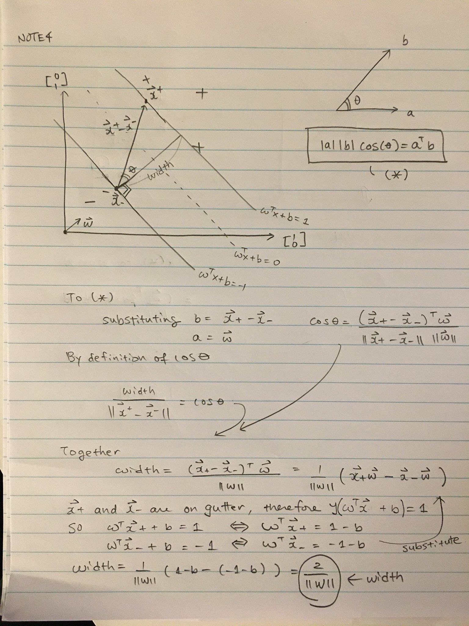
Remind you that we need to maximize the margin, or the distance of the two lines as far as possible. Let's try to find the distance between the two separating lines.
You can show that the width, defined by the two observations on the gutters, are in fact
$$ \textrm{width} = \frac{2}{|| \boldsymbol{w}||} $$
Optimization
The weights that maximizing width is the same as the weights that minimizes $$ \frac{1}{2}|| \boldsymbol{w}||^2 $$ This minimization must be done under the constraint of
$$ y_i(\boldsymbol{w}\boldsymbol{x}_{i} + b) \ge 1 \\ $$
while those observations on gutters must satisfy:
\begin{array}{rl} y_i (\boldsymbol{w}\boldsymbol{x}_{gutter} + b) = 1 \\ \end{array}
This is done by Lagrange multiplier $\alpha_i$. The optimization problem becomes:
$$ L(\boldsymbol{w}) = \frac{1}{2}|| \boldsymbol{w}||^2 - \sum_{i=1}^N \alpha_i\left( y_i (\boldsymbol{w}\boldsymbol{x}_i+ b) - 1\right) $$
Fact:
- Only some of the $\alpha_i$ on gutters receive nonzero values in this optimization problem!!!
The first derivative is:
$$ \frac{\partial L(\boldsymbol{w})}{\partial \boldsymbol{w}} =\boldsymbol{w} - \sum_{i=1}^N \alpha_i y_i \boldsymbol{x}_i = 0 $$
So $$ \boldsymbol{w} = \sum_{i=1}^N \alpha_i y_i \boldsymbol{x}_i $$
$$ \frac{\partial L(\boldsymbol{w})}{\partial \boldsymbol{b}} = \sum_{i=1}^N \alpha_i y_i = 0 $$
$L(\alpha_i,i=1,\cdots, N)$
Substitute these to $L(\boldsymbol{w})$ and see how $L(\boldsymbol{w})$ can be represented with respect to $\alpha_i$.
\begin{array}{rl} L(\alpha_i,i=1,\cdots, N)& = \frac{1}{2} \sum_{i=1}^N \alpha_i y_i \boldsymbol{x}_i^T \sum_{i=1}^N \alpha_i y_i \boldsymbol{x}_i - \sum_{i=1}^N \alpha_i y_i \left( \sum_{k=1}^N \alpha_k y_k \boldsymbol{x}_k\right)\boldsymbol{x}_i+ b \sum_{i=1}^N \alpha_i y_i - \sum_{i=1}^N \alpha_i \\ & = \sum_{i=1}^N \alpha_i -\frac{1}{2} \sum_{i=1}^N \sum_{j=1}^N \alpha_i\alpha_j y_i y_j \boldsymbol{x}_i^T \boldsymbol{x}_j \end{array}
This representation shows that the observations $\boldsymbol{x}_i$ comes into play in the loss function only as a pair.
Therefore, when you define kernel to add complexity, Kernel only needs to define the distance of the pair of the observations.
The decision rule also only depends on the dot products!