In this blog, I will follow Recommendations in TensorFlow: Create the Model and study basic yet powerful recommendation algorithm, collaborative filtering using tensorflow version 1.
What you learn
- collaborative filtering
- Weighted alternating least squares (WALS) method
- tensorflow (v1.15.0)
In particular, this blog will show that the WALS method is pretty sensitive to the choice of weights (linear weights v.s. log weights vs uniform weights). I will use movieLens 100k
Multidimensional indexing with tensorflow
In this blog post, I present how to use multi-dimensional index arrays for indexing tensors.
First, I will show multi-dimensional array indexing with numpy. Then I will show two approaches in tensorflow:
- tf.while_loop
- tf.gather_nd
I will conclude that tf.gather_nd is much more effective than tf.while_loop.
Reference
Classification with Mahalanobis distance + full covariance using tensorflow
This blog discusses how to calculate Mahalanobis distance using tensorflow. I will consider full variance approach, i.e., each cluster has its own general covariance matrix, so I do not assume common variance accross clusters unlike the previous post. Calculation of Mahalanobis distance is important for classification when each cluster has different covariance structure. Let's take a lookt at this situation using toy data.
Calculate Mahalanobis distance with tensorflow 2.0
I noticed that tensorflow does not have functions to compute Mahalanobis distance between two groups of samples. So here I go and provide the code with explanation. The blog is organized and explain the following topics
- Euclidean distance with Scipy
- Euclidean distance with Tensorflow v2
- Mahalanobis distance with Scipy
- Mahalanobis distance with Tensorflow v2
Sample size calculation to predict proportion of fake accounts in social media
Introduction
How many sample do you need to predict the proportion of fake account in a social network?
Obviously, if human manually check every account one by one for ALL the accounts in the social network, we can get the actual proportion of the fake accounts. But this would be too expensive and time consuming, especially when social accounts nowadays contain billions of active accounts! Facebook has 2 billion users, LinkedIn has .5 billion users.
Gentle Hands-on Introduction to Propensity Score Matching
Introduction
Data Scientists need to help making business decisions by providing insights from data. To answer to the questions like "does a new feature improve user engagement?", data scientists may conduct A/B testing to see if there is any "causal" effect of new feature on user's engagement, evaluated with certain metric. Before diving into causal inference in observational study, let's talk about more common approach: A/B testing and its limitation.
Inverse transform sampling and other sampling techniques
Random number generation is important techniques in various statistical modeling, for example, to create Markov Chain Monte Carlo algorithm, or simple Monte Carlo simulation. Here, I make notes on some standard sampling techiniques, and demonstrate its useage in R.
Inverse Transform Sampling
Inverse Transform Sampling is a powerful sampling technique because you can generate samples from any distribution with this technique, as long as its cumulative distribution function exists.
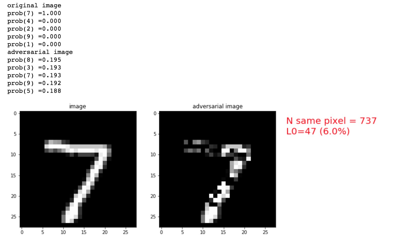
Learn the Carlini and Wagner's adversarial attack - MNIST

Deep neural networks (DNN) have become increasingly effective at many difficult machine-learning tasks. However, DNNs are vulnerable to adversarial examples that are maliciously made to misguide the DNN's performance. The vulnerability may make it difficult to apply the DNNs to security sensitive usecases. In this blog, we learn one of the most successful adversarial attack proposed in the paper "Toward Evaluating the Robustness of Neural Network".
What would happen if image is analyzed with 1D-DCT vs 2D-DCT?
In the previous blog, I reviewed 1D-DCT and 2D-DCT. In this blog, I will check what would happen if you denoise the image via 1D-DCT on flattened image.
Denoising
I will denoise the image by first transforming an image to frequency domain and pick the top $k$ largest DCT coefficients in absolute values. The remaining DCT coefficients are sparcified to zero. The new DCT coefficients are then inverse DCTed to spacial domain. The recovered image is visualized.
Two-dimensional Discrete Cosine Transform as a Linear Transformation
In previous blog post I reviewed one-dimensional Discrete Fourier Transform (DFT) as well as two-dimensional DFT. This short post is along the same line, and specifically study the following topics:
- Discrete Cosine Transform
- Represent DCT as a linear transformation of measurements in time/spatial domain to the frequency domain.
- What would happen if you use 1D DFT on the image, which has two dimensions?