Yumi's Blog

Achieving top 5 in Kaggle's facial keypoints detection using FCN

final submission screen shot

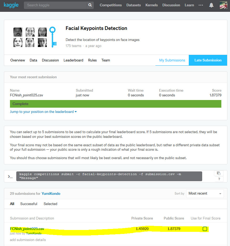
My Kaggle's final score using the model explained in this ipython notebook.

In [1]:
from IPython.display import IFrame
src = "https://www.youtube.com/embed/8FdSHl4oNIM" 
IFrame(src, width=990/2, height=800/2)
Out[1]:

A few days ago, I saw this very awesome youtube video demonstrating the performance of the state-of-art facial keypoint detection. This video was a part of ICCV 2017's presentation How far are we from solving the 2D & 3D Face Alignment problem? (and a dataset of 230,000 3D facial landmarks).

This paper says that the current state-of-art landmark localization problem uses Hour-Glass network of Stacked Hourglass Networks for Human Pose Estimation. Hour-Glass network uses the idea from the fully convolutional networks, which is often used in object segmentation task. I also studied FCN in previous blog using object segmentation data. Here, I was originally confused about how to apply the model from the object segmentation task to the facial landmark detection task. The data structure of the two problems are quite different:

  • facial landmark detection:
    • input: image
    • output: x,y coordinate of landmarks
  • object segmentation:
    • input: image
    • output: the object's class at every pixcel

For example in my previous blog, Achieving Top 23% in Kaggle's Facial Keypoints Detection with Keras + Tensorflow, I did a facial keypoints (landmarks) detection using Kaggle's facial keypoints detection data. In this post, I used CNN to extract features and then regress on the x,y coordinates of the landmarks.

So how can we apply the model from the object segmentation to the facial landmark detection problem? The answer was in the preprocessing of images: the (x,y)-coordinates of the landmarks are transformed to "heatmap" using some kernels e.g. Gaussian kernel. Then the problem becomes estimating the value of the heatmap at every pixcel just like object detection problem where the goal is to estimate the object's class at every pixcel. Interesting!

In this blog post, I will revisit Kaggle's facial keypoints detection data to learn the performance of simple FCN-like model for the facial keypoint detection problem.

I was able to improve the private and public scores of this competition from my previous model. The script here can yield:

  • Private score : 1.45920
  • Public score : 1.87379

This means that I am "roughly" in Top 5 in the private score and Top 6 in the public score out of 175 teams. I use the word "roughly" because the competition has ended in January 2017, and final scores are not available for me. (The final offical scores are evaluated using 50% of the testing data while the results here are based on ALL the testing data. Nevertheless, the model performance is pretty good.

Import libraries

In [2]:
import matplotlib.pyplot as plt
import tensorflow as tf
from keras.backend.tensorflow_backend import set_session
import keras, sys, time, os, warnings, cv2

from keras.models import *
from keras.layers import *

import numpy as np
import pandas as pd 
warnings.filterwarnings("ignore")


os.environ["CUDA_DEVICE_ORDER"] = "PCI_BUS_ID" 
config = tf.ConfigProto()
config.gpu_options.per_process_gpu_memory_fraction = 0.95
config.gpu_options.visible_device_list = "1" 
set_session(tf.Session(config=config))   


print("python {}".format(sys.version))
print("keras version {}".format(keras.__version__)); del keras
print("tensorflow version {}".format(tf.__version__))
Using TensorFlow backend.
python 2.7.13 |Anaconda 4.3.1 (64-bit)| (default, Dec 20 2016, 23:09:15) 
[GCC 4.4.7 20120313 (Red Hat 4.4.7-1)]
keras version 2.0.6
tensorflow version 1.2.1

The data is downloaded from Kaggle's facial keypoints detection, and saved under data folder.

In [3]:
FTRAIN = "data/training.csv"
FTEST  = "data/test.csv"
FIdLookup = 'data/IdLookupTable.csv'

Data importing and preprocessing

Create a Gaussian heatmap

I will use the data loading functions from Achieving Top 23% in Kaggle's Facial Keypoints Detection with Keras + Tensorflow with some modifications that transform each (x,y)-coordinate facial keypoint to a single heatmap using Gaussian kernel. For example, in Kaggle's facial keypoints detection problem, there are 15 facial keypoints to estimate. So this means that I will create 15 heatmaps.

In the case of left eye landmark, the Gaussian kernel centered around left eye landmark $( x_{\textrm{left eye landmark}}, y_{\textrm{left eye landmark}})$ has a value at ($x,y$) as:

$$ \frac{1}{2\pi \sigma^2 } exp \left({-\frac{(x-x_{\textrm{left eye landmark}})^2 + (y-y_{\textrm{left eye landmark}})^2}{2 \sigma^2}}\right) = constant * \left({-\frac{(x-x_{\textrm{left eye landmark}})^2 + (y-y_{\textrm{left eye landmark}})^2}{2 \sigma^2}}\right) $$

I need to pre-specify $\sigma^2$ as a hyper parameter. I found that the choice of $\sigma^2$ is important to get sensible results. If $\sigma^2$ is too low, the heatmap becomes too sparse (mostly zero) for a model to train. If $\sigma^2$ is too high, the trained model focuses too much on estimating the magnitude of non-landmark coordinates.

The constant scale is another hyper parameter that also needs to be adjusted via, e.g., cross-validation.

The following functions are for transforming (x,y)-coordinate of a landmark to a heatmap.

In [4]:
def gaussian_k(x0,y0,sigma, width, height):
        """ Make a square gaussian kernel centered at (x0, y0) with sigma as SD.
        """
        x = np.arange(0, width, 1, float) ## (width,)
        y = np.arange(0, height, 1, float)[:, np.newaxis] ## (height,1)
        return np.exp(-((x-x0)**2 + (y-y0)**2) / (2*sigma**2))

def generate_hm(height, width ,landmarks,s=3):
        """ Generate a full Heap Map for every landmarks in an array
        Args:
            height    : The height of Heat Map (the height of target output)
            width     : The width  of Heat Map (the width of target output)
            joints    : [(x1,y1),(x2,y2)...] containing landmarks
            maxlenght : Lenght of the Bounding Box
        """
        Nlandmarks = len(landmarks)
        hm = np.zeros((height, width, Nlandmarks), dtype = np.float32)
        for i in range(Nlandmarks):
            if not np.array_equal(landmarks[i], [-1,-1]):
             
                hm[:,:,i] = gaussian_k(landmarks[i][0],
                                        landmarks[i][1],
                                        s,height, width)
            else:
                hm[:,:,i] = np.zeros((height,width))
        return hm
    
def get_y_as_heatmap(df,height,width, sigma):
    
    columns_lmxy = df.columns[:-1] ## the last column contains Image
    columns_lm = [] 
    for c in columns_lmxy:
        c = c[:-2]
        if c not in columns_lm:
            columns_lm.extend([c])
    
    y_train = []
    for i in range(df.shape[0]):
        landmarks = []
        for colnm in columns_lm:
            x = df[colnm + "_x"].iloc[i]
            y = df[colnm + "_y"].iloc[i]
            if np.isnan(x) or np.isnan(y):
                x, y = -1, -1
            landmarks.append([x,y])
            
        y_train.append(generate_hm(height, width, landmarks, sigma))
    y_train = np.array(y_train)
    
    
    return(y_train,df[columns_lmxy],columns_lmxy)

Functions to extract, transfer and load data

These functions are very similar to the ones from Achieving Top 23% in Kaggle's Facial Keypoints Detection with Keras + Tensorflow.

In [5]:
def load(test=False, width=96,height=96,sigma=5):
    """
    load test/train data
    cols : a list containing landmark label names.
           If this is specified, only the subset of the landmark labels are 
           extracted. for example, cols could be:
           
          [left_eye_center_x, left_eye_center_y]
            
    return: 
    X:  2-d numpy array (Nsample, Ncol*Nrow)
    y:  2-d numpy array (Nsample, Nlandmarks*2) 
        In total there are 15 landmarks. 
        As x and y coordinates are recorded, u.shape = (Nsample,30)
    y0: panda dataframe containins the landmarks
       
    """
    from sklearn.utils import shuffle
    
    fname = FTEST if test else FTRAIN
    df = pd.read_csv(os.path.expanduser(fname)) 

    
    df['Image'] = df['Image'].apply(lambda im: np.fromstring(im, sep=' '))


    myprint = df.count()
    myprint = myprint.reset_index()
    print(myprint)  
    ## row with at least one NA columns are removed!
    ## df = df.dropna()  
    df = df.fillna(-1)

    X = np.vstack(df['Image'].values) / 255.  # changes valeus between 0 and 1
    X = X.astype(np.float32)

    if not test:  # labels only exists for the training data
        y, y0, nm_landmark = get_y_as_heatmap(df,height,width, sigma)
        X, y, y0 = shuffle(X, y, y0, random_state=42)  # shuffle data   
        y = y.astype(np.float32)
    else:
        y, y0, nm_landmark = None, None, None
    
    return X, y, y0, nm_landmark

def load2d(test=False,width=96,height=96,sigma=5):

    re   = load(test,width,height,sigma)
    X    = re[0].reshape(-1,width,height,1)
    y, y0, nm_landmarks = re[1:]
    
    return X, y, y0, nm_landmarks

Import training data and testing data

In [6]:
sigma = 5

X_train, y_train, y_train0, nm_landmarks = load2d(test=False,sigma=sigma)
X_test,  y_test, _, _ = load2d(test=True,sigma=sigma)
print X_train.shape,y_train.shape, y_train0.shape
print X_test.shape,y_test
                        index     0
0           left_eye_center_x  7039
1           left_eye_center_y  7039
2          right_eye_center_x  7036
3          right_eye_center_y  7036
4     left_eye_inner_corner_x  2271
5     left_eye_inner_corner_y  2271
6     left_eye_outer_corner_x  2267
7     left_eye_outer_corner_y  2267
8    right_eye_inner_corner_x  2268
9    right_eye_inner_corner_y  2268
10   right_eye_outer_corner_x  2268
11   right_eye_outer_corner_y  2268
12   left_eyebrow_inner_end_x  2270
13   left_eyebrow_inner_end_y  2270
14   left_eyebrow_outer_end_x  2225
15   left_eyebrow_outer_end_y  2225
16  right_eyebrow_inner_end_x  2270
17  right_eyebrow_inner_end_y  2270
18  right_eyebrow_outer_end_x  2236
19  right_eyebrow_outer_end_y  2236
20                 nose_tip_x  7049
21                 nose_tip_y  7049
22        mouth_left_corner_x  2269
23        mouth_left_corner_y  2269
24       mouth_right_corner_x  2270
25       mouth_right_corner_y  2270
26     mouth_center_top_lip_x  2275
27     mouth_center_top_lip_y  2275
28  mouth_center_bottom_lip_x  7016
29  mouth_center_bottom_lip_y  7016
30                      Image  7049
     index     0
0  ImageId  1783
1    Image  1783
(7049, 96, 96, 1) (7049, 96, 96, 15) (7049, 30)
(1783, 96, 96, 1) None

Visualize original gray scale image together with heatmap

Some of the heatmaps are just black indicating that some landmarks are not recorded (missing), and all the pixcels from this heatmap are zero.

In principle, my deep learning model can accept all-zero heatmap and handle the missing landmarks with no extra effort. Such approach may be approriate if the landmark does not exist in the image: For example, if the left eye is outside of the image, the heatmap for the left eye should be all zero (while the heatmaps of other landmarks from the same image may or may not be all zeros).

However, in this Kaggle's data, I see that all landmarks exist within the image, but for some reasons, some landmark's (x,y) coordinates are not recorded. See plotted images below. So, using all-zero heatmap in training gives misleading infomation to the model; there is no landmark in the image while there is! We should treat these "missing" (x,y)-coordinate landmarks as mis-labeled or contaminated data, and simply do not use such landmarks in training. This can be achieved using weights, and presented later.

In [7]:
Nplot = y_train.shape[3]+1

for i in range(3):
    fig = plt.figure(figsize=(20,6))
    ax = fig.add_subplot(2,Nplot/2,1)
    ax.imshow(X_train[i,:,:,0],cmap="gray")
    ax.set_title("input")
    for j, lab in enumerate(nm_landmarks[::2]):
        ax = fig.add_subplot(2,Nplot/2,j+2)
        ax.imshow(y_train[i,:,:,j],cmap="gray")
        ax.set_title(str(j) +"\n" + lab[:-2] )
    plt.show()

Data augmentation

My previous blog showed that it is very important to augment the available training images to improve the model performance on future, validation data.

The code below can do wide range of affine transformation and horizontal flipping. Note that the horizontal flipping in the landmark detection problem needs to make sure that the left-XX label and rand-XX labels are also flipped. In this Kaggle competition, we have 15 landmarks. For example, when horizontal flip happens the left_eye_center (0th landmark) needs to be swapped to the right_eye_center. To keep track on which pairs of landmarks to be swapped, we introduce a dictionary recording the original and new landmark's index:

landmark_order = {"orig" : [0,1,2,3,4,5,6,7,8,9,11,12],
                  "new"  : [1,0,4,5,2,3,8,9,6,7,12,11]}

In my model, I uses weights and horizontal swap will affects the order of weights. This point will become more clear later in the code.

Note: the data augmentation function is not optimized and it sustantially increase the training time :\

Functions

In [8]:
from skimage import transform
from skimage.transform import SimilarityTransform, AffineTransform
import random 


def transform_img(data,
                  loc_w_batch=2,
                  max_rotation=0.01,
                  max_shift=2,
                  max_shear=0,
                  max_scale=0.01,mode="edge"):
    '''
    data : list of numpy arrays containing a single image
    e.g., data = [X, y, w] or data = [X, y]
    X.shape = (height, width, NfeatX)
    y.shape = (height, width, Nfeaty)
    w.shape = (height, width, Nfeatw)
    NfeatX, Nfeaty and Nfeatw can be different
    
    affine transformation for a single image
    
    loc_w_batch : the location of the weights in the fourth dimention
    [,,,loc_w_batch]
    '''
    scale = (np.random.uniform(1-max_scale, 1 + max_scale),
             np.random.uniform(1-max_scale, 1 + max_scale))
    rotation_tmp = np.random.uniform(-1*max_rotation, max_rotation)
    translation = (np.random.uniform(-1*max_shift, max_shift),
                   np.random.uniform(-1*max_shift, max_shift))
    shear = np.random.uniform(-1*max_shear, max_shear)
    tform = AffineTransform(
            scale=scale,#,
            ## Convert angles from degrees to radians.
            rotation=np.deg2rad(rotation_tmp),
            translation=translation,
            shear=np.deg2rad(shear)
        )
    
    for idata, d in enumerate(data):
        if idata != loc_w_batch:
            ## We do NOT need to do affine transformation for weights
            ## as weights are fixed for each (image,landmark) combination
            data[idata] = transform.warp(d, tform,mode=mode)
    return data
def transform_imgs(data, lm, 
                   loc_y_batch = 1, 
                   loc_w_batch = 2):
    '''
    data : list of numpy arrays containing a single image
    e.g., data = [X, y, w] or data = [X, y]
    X.shape = (height, width, NfeatX)
    y.shape = (height, width, Nfeaty)
    w.shape = (height, width, Nfeatw)
    NfeatX, Nfeaty and Nfeatw can be different
    
    affine transformation for a single image
    '''
    Nrow  = data[0].shape[0]
    Ndata = len(data) 
    data_transform = [[] for i in range(Ndata)]
    for irow in range(Nrow):
        data_row = []
        for idata in range(Ndata):
            data_row.append(data[idata][irow])
        ## affine transformation
        data_row_transform = transform_img(data_row,
                                          loc_w_batch)
        ## horizontal flip
        data_row_transform = horizontal_flip(data_row_transform,
                                             lm,
                                             loc_y_batch,
                                             loc_w_batch)
        
        for idata in range(Ndata):
            data_transform[idata].append(data_row_transform[idata])
    
    for idata in range(Ndata):
        data_transform[idata] = np.array(data_transform[idata])
    
    
    return(data_transform)

def horizontal_flip(data,lm,loc_y_batch=1,loc_w_batch=2):  
    '''
    flip the image with 50% chance
    
    lm is a dictionary containing "orig" and "new" key
    This must indicate the potitions of heatmaps that need to be flipped  
    landmark_order = {"orig" : [0,1,2,3,4,5,6,7,8,9,11,12],
                      "new"  : [1,0,4,5,2,3,8,9,6,7,12,11]}
                      
    data = [X, y, w]
    w is optional and if it is in the code, the position needs to be specified
    with loc_w_batch
    
    X.shape (height,width,n_channel)
    y.shape (height,width,n_landmarks)
    w.shape (height,width,n_landmarks)
    '''
    lo, ln = np.array(lm["orig"]), np.array(lm["new"])

    assert len(lo) == len(ln)
    if np.random.choice([0,1]) == 1:
        return(data)
    
    for i, d in enumerate(data):
        d = d[:, ::-1,:] 
        data[i] = d


    data[loc_y_batch] = swap_index_for_horizontal_flip(
        data[loc_y_batch], lo, ln)

    # when horizontal flip happens to image, we need to heatmap (y) and weights y and w
    # do this if loc_w_batch is within data length
    if loc_w_batch < len(data):
        data[loc_w_batch] = swap_index_for_horizontal_flip(
            data[loc_w_batch], lo, ln)
    return(data)

def swap_index_for_horizontal_flip(y_batch, lo, ln):
    '''
    lm = {"orig" : [0,1,2,3,4,5,6,7,8,9,11,12],
          "new"  : [1,0,4,5,2,3,8,9,6,7,12,11]}
    lo, ln = np.array(lm["orig"]), np.array(lm["new"])                  
    '''
    y_orig = y_batch[:,:, lo]
    y_batch[:,:, lo] = y_batch[:,:, ln] 
    y_batch[:,:, ln] = y_orig
    return(y_batch)

Visualizing augmented images

Notice that the image is shifted and also horizontally flipped in random fashion. When horizontal flip happens, the right eye is labeled as left eye and vise versa.

In [9]:
## example image to  visualize the data augmentation
iexample = 139
## Show the first 13 heatmaps
Nhm = 10

plt.imshow(X_train[iexample,:,:,0],cmap="gray")
plt.title("original")
plt.axis("off")
plt.show()
Nplot = 5
fig = plt.figure(figsize=[Nhm*2.5,2*Nplot])


landmark_order = {"orig" : [0,1,2,3,4,5,6,7,8,9,11,12],
                  "new"  : [1,0,4,5,2,3,8,9,6,7,12,11]}


count = 1
for _ in range(Nplot):
    x_batch, y_batch = transform_imgs([X_train[[iexample]],
                                       y_train[[iexample]]],
                                     landmark_order)
    ax = fig.add_subplot(Nplot,Nhm+1,count)
    ax.imshow(x_batch[0,:,:,0],cmap="gray")
    ax.axis("off")
    count += 1 
    
    for ifeat in range(Nhm):
        ax = fig.add_subplot(Nplot,Nhm + 1,count)
        ax.imshow(y_batch[0,:,:,ifeat],cmap="gray")
        ax.axis("off")
        if count < Nhm + 2:
            ax.set_title(nm_landmarks[ifeat*2][:-2])
        count += 1
plt.show()

Split data into training and validation data

In [10]:
prop_train = 0.9
Ntrain = int(X_train.shape[0]*prop_train)
X_tra, y_tra, X_val,y_val = X_train[:Ntrain],y_train[:Ntrain],X_train[Ntrain:],y_train[Ntrain:]
del X_train, y_train

Define FCN-like model

This model is simplified version of FCN8. See my previous blog post about FCN8.

In [11]:
input_height, input_width = 96, 96
## output shape is the same as input
output_height, output_width = input_height, input_width 
n = 32*5
nClasses = 15
nfmp_block1 = 64
nfmp_block2 = 128

IMAGE_ORDERING =  "channels_last" 
img_input = Input(shape=(input_height,input_width, 1)) 

# Encoder Block 1
x = Conv2D(nfmp_block1, (3, 3), activation='relu', padding='same', name='block1_conv1', data_format=IMAGE_ORDERING )(img_input)
x = Conv2D(nfmp_block1, (3, 3), activation='relu', padding='same', name='block1_conv2', data_format=IMAGE_ORDERING )(x)
block1 = MaxPooling2D((2, 2), strides=(2, 2), name='block1_pool', data_format=IMAGE_ORDERING )(x)
    
# Encoder Block 2
x = Conv2D(nfmp_block2, (3, 3), activation='relu', padding='same', name='block2_conv1', data_format=IMAGE_ORDERING )(block1)
x = Conv2D(nfmp_block2, (3, 3), activation='relu', padding='same', name='block2_conv2', data_format=IMAGE_ORDERING )(x)
x = MaxPooling2D((2, 2), strides=(2, 2), name='block2_pool', data_format=IMAGE_ORDERING )(x)
    
## bottoleneck    
o = (Conv2D(n, (input_height/4, input_width/4), 
            activation='relu' , padding='same', name="bottleneck_1", data_format=IMAGE_ORDERING))(x)
o = (Conv2D(n , ( 1 , 1 ) , activation='relu' , padding='same', name="bottleneck_2", data_format=IMAGE_ORDERING))(o)


## upsamping to bring the feature map size to be the same as the one from block1
## o_block1 = Conv2DTranspose(nfmp_block1, kernel_size=(2,2),  strides=(2,2), use_bias=False, name='upsample_1', data_format=IMAGE_ORDERING )(o)
## o = Add()([o_block1,block1])
## output   = Conv2DTranspose(nClasses,    kernel_size=(2,2),  strides=(2,2), use_bias=False, name='upsample_2', data_format=IMAGE_ORDERING )(o)

## Decoder Block
## upsampling to bring the feature map size to be the same as the input image i.e., heatmap size
output   = Conv2DTranspose(nClasses,    kernel_size=(4,4),  strides=(4,4), use_bias=False, name='upsample_2', data_format=IMAGE_ORDERING )(o)

## Reshaping is necessary to use sample_weight_mode="temporal" which assumes 3 dimensional output shape
## See below for the discussion of weights
output = Reshape((output_width*input_height*nClasses,1))(output)
model = Model(img_input, output)
model.summary()

model.compile(loss='mse',optimizer="rmsprop",sample_weight_mode="temporal")
_________________________________________________________________
Layer (type)                 Output Shape              Param #   
=================================================================
input_1 (InputLayer)         (None, 96, 96, 1)         0         
_________________________________________________________________
block1_conv1 (Conv2D)        (None, 96, 96, 64)        640       
_________________________________________________________________
block1_conv2 (Conv2D)        (None, 96, 96, 64)        36928     
_________________________________________________________________
block1_pool (MaxPooling2D)   (None, 48, 48, 64)        0         
_________________________________________________________________
block2_conv1 (Conv2D)        (None, 48, 48, 128)       73856     
_________________________________________________________________
block2_conv2 (Conv2D)        (None, 48, 48, 128)       147584    
_________________________________________________________________
block2_pool (MaxPooling2D)   (None, 24, 24, 128)       0         
_________________________________________________________________
bottleneck_1 (Conv2D)        (None, 24, 24, 160)       11796640  
_________________________________________________________________
bottleneck_2 (Conv2D)        (None, 24, 24, 160)       25760     
_________________________________________________________________
upsample_2 (Conv2DTranspose) (None, 96, 96, 15)        38400     
_________________________________________________________________
reshape_1 (Reshape)          (None, 138240, 1)         0         
=================================================================
Total params: 12,119,808
Trainable params: 12,119,808
Non-trainable params: 0
_________________________________________________________________

Sample weights

We will only include the annotated landmarks to calculate the loss.

To do this, I will define the weight matrix (N_image, height, width, N_landmark). In this weight matrix, if the (x,y)-coordinate of the landmark of the image is recorded, all the height x width pixcels have value 1, and if the landmark is not recorded, all the pixcels have value 0.

Keras acepts the weight matrix to be at most 2 dimensional at this moment (May 2018) with the first dimension corresponding to the image sample. We reshape the weight matrix into the size (N_image, height x width x N_landmark).

In [12]:
def find_weight(y_tra):
    '''
    :::input:::
    
    y_tra : np.array of shape (N_image, height, width, N_landmark)
    
    :::output::: 
    
    weights : 
        np.array of shape (N_image, height, width, N_landmark)
        weights[i_image, :, :, i_landmark] = 1 
                        if the (x,y) coordinate of the landmark for this image is recorded.
        else  weights[i_image, :, :, i_landmark] = 0

    '''
    weight = np.zeros_like(y_tra)
    count0, count1 = 0, 0
    for irow in range(y_tra.shape[0]):
        for ifeat in range(y_tra.shape[-1]):
            if np.all(y_tra[irow,:,:,ifeat] == 0):
                value = 0
                count0 += 1
            else:
                value = 1
                count1 += 1
            weight[irow,:,:,ifeat] = value
    print("N landmarks={:5.0f}, N missing landmarks={:5.0f}, weight.shape={}".format(
        count0,count1,weight.shape))
    return(weight)


def flatten_except_1dim(weight,ndim=2):
    '''
    change the dimension from:
    (a,b,c,d,..) to (a, b*c*d*..) if ndim = 2
    (a,b,c,d,..) to (a, b*c*d*..,1) if ndim = 3
    '''
    n = weight.shape[0]
    if ndim == 2:
        shape = (n,-1)
    elif ndim == 3:
        shape = (n,-1,1)
    else:
        print("Not implemented!")
    weight = weight.reshape(*shape)
    return(weight)

Define weights for training, and validation data.

In [13]:
w_tra = find_weight(y_tra)

weight_val = find_weight(y_val)
weight_val = flatten_except_1dim(weight_val)
y_val_fla  = flatten_except_1dim(y_val,ndim=3) 

## print("weight_tra.shape={}".format(weight_tra.shape))
print("weight_val.shape={}".format(weight_val.shape))
print("y_val_fla.shape={}".format(y_val_fla.shape))
print(model.output.shape)
N landmarks=47185, N missing landmarks=47975, weight.shape=(6344, 96, 96, 15)
N landmarks= 5521, N missing landmarks= 5054, weight.shape=(705, 96, 96, 15)
weight_val.shape=(705, 138240)
y_val_fla.shape=(705, 138240, 1)
(?, 138240, 1)

Training starts here!

In [14]:
nb_epochs = 300
batch_size = 32
const = 10 
history = {"loss":[],"val_loss":[]}
for iepoch in range(nb_epochs):
    start = time.time()
    
    
    x_batch, y_batch, w_batch = transform_imgs([X_tra,y_tra, w_tra],landmark_order)
    # If you want no data augementation, comment out the line above and uncomment the comment below:
    # x_batch, y_batch, w_batch = X_tra,y_tra, w_batch 
    w_batch_fla = flatten_except_1dim(w_batch,ndim=2)
    y_batch_fla = flatten_except_1dim(y_batch,ndim=3)
    
    hist = model.fit(x_batch,
                     y_batch_fla*const,
                     sample_weight = w_batch_fla,
                     validation_data=(X_val,y_val_fla*const,weight_val),
                     batch_size=batch_size,
                     epochs=1,
                     verbose=0)
    history["loss"].append(hist.history["loss"][0])
    history["val_loss"].append(hist.history["val_loss"][0])
    end = time.time()
    print("Epoch {:03}: loss {:6.4f} val_loss {:6.4f} {:4.1f}sec".format(
        iepoch+1,history["loss"][-1],history["val_loss"][-1],end-start))
Epoch 001: loss 0.4608 val_loss 0.2802 89.4sec
Epoch 002: loss 0.2289 val_loss 0.2765 80.2sec
Epoch 003: loss 0.1768 val_loss 0.1417 81.1sec
Epoch 004: loss 0.1492 val_loss 0.2057 83.9sec
Epoch 005: loss 0.1332 val_loss 0.1253 79.8sec
Epoch 006: loss 0.1221 val_loss 0.1518 81.5sec
Epoch 007: loss 0.1125 val_loss 0.1188 80.1sec
Epoch 008: loss 0.1056 val_loss 0.1164 81.4sec
Epoch 009: loss 0.0998 val_loss 0.0939 81.5sec
Epoch 010: loss 0.0940 val_loss 0.0916 82.0sec
Epoch 011: loss 0.0903 val_loss 0.0937 79.0sec
Epoch 012: loss 0.0858 val_loss 0.1134 80.8sec
Epoch 013: loss 0.0825 val_loss 0.1103 80.1sec
Epoch 014: loss 0.0791 val_loss 0.0719 79.8sec
Epoch 015: loss 0.0756 val_loss 0.0909 80.1sec
Epoch 016: loss 0.0734 val_loss 0.0917 80.2sec
Epoch 017: loss 0.0709 val_loss 0.0763 79.9sec
Epoch 018: loss 0.0686 val_loss 0.0823 79.2sec
Epoch 019: loss 0.0664 val_loss 0.0753 80.6sec
Epoch 020: loss 0.0642 val_loss 0.0891 81.2sec
Epoch 021: loss 0.0626 val_loss 0.0768 80.1sec
Epoch 022: loss 0.0609 val_loss 0.0812 80.3sec
Epoch 023: loss 0.0592 val_loss 0.0765 80.6sec
Epoch 024: loss 0.0576 val_loss 0.0755 82.7sec
Epoch 025: loss 0.0562 val_loss 0.0698 79.8sec
Epoch 026: loss 0.0545 val_loss 0.0773 82.5sec
Epoch 027: loss 0.0532 val_loss 0.0711 85.0sec
Epoch 028: loss 0.0522 val_loss 0.0747 82.3sec
Epoch 029: loss 0.0510 val_loss 0.0751 81.4sec
Epoch 030: loss 0.0496 val_loss 0.0743 81.3sec
Epoch 031: loss 0.0485 val_loss 0.0926 81.4sec
Epoch 032: loss 0.0475 val_loss 0.0765 80.4sec
Epoch 033: loss 0.0465 val_loss 0.0747 80.9sec
Epoch 034: loss 0.0458 val_loss 0.0723 81.7sec
Epoch 035: loss 0.0448 val_loss 0.0720 81.7sec
Epoch 036: loss 0.0441 val_loss 0.0715 82.3sec
Epoch 037: loss 0.0432 val_loss 0.0759 81.7sec
Epoch 038: loss 0.0424 val_loss 0.0796 81.7sec
Epoch 039: loss 0.0417 val_loss 0.0741 81.8sec
Epoch 040: loss 0.0406 val_loss 0.0709 81.0sec
Epoch 041: loss 0.0400 val_loss 0.0727 81.8sec
Epoch 042: loss 0.0394 val_loss 0.0722 82.0sec
Epoch 043: loss 0.0391 val_loss 0.0759 82.5sec
Epoch 044: loss 0.0384 val_loss 0.0787 82.0sec
Epoch 045: loss 0.0378 val_loss 0.0726 81.7sec
Epoch 046: loss 0.0370 val_loss 0.0775 86.2sec
Epoch 047: loss 0.0370 val_loss 0.0753 82.1sec
Epoch 048: loss 0.0364 val_loss 0.0780 82.0sec
Epoch 049: loss 0.0356 val_loss 0.0732 81.6sec
Epoch 050: loss 0.0351 val_loss 0.0707 81.7sec
Epoch 051: loss 0.0347 val_loss 0.0749 81.5sec
Epoch 052: loss 0.0343 val_loss 0.0781 82.6sec
Epoch 053: loss 0.0336 val_loss 0.0764 81.3sec
Epoch 054: loss 0.0334 val_loss 0.0897 82.1sec
Epoch 055: loss 0.0333 val_loss 0.0705 81.7sec
Epoch 056: loss 0.0328 val_loss 0.0752 83.1sec
Epoch 057: loss 0.0325 val_loss 0.0741 81.3sec
Epoch 058: loss 0.0320 val_loss 0.0715 81.8sec
Epoch 059: loss 0.0318 val_loss 0.0709 81.7sec
Epoch 060: loss 0.0313 val_loss 0.0678 81.8sec
Epoch 061: loss 0.0311 val_loss 0.0710 81.8sec
Epoch 062: loss 0.0308 val_loss 0.0707 82.8sec
Epoch 063: loss 0.0306 val_loss 0.0723 83.9sec
Epoch 064: loss 0.0301 val_loss 0.0771 81.0sec
Epoch 065: loss 0.0299 val_loss 0.0726 81.7sec
Epoch 066: loss 0.0296 val_loss 0.0691 82.6sec
Epoch 067: loss 0.0296 val_loss 0.0743 82.2sec
Epoch 068: loss 0.0290 val_loss 0.0762 82.4sec
Epoch 069: loss 0.0287 val_loss 0.0749 81.8sec
Epoch 070: loss 0.0288 val_loss 0.0741 81.1sec
Epoch 071: loss 0.0284 val_loss 0.0707 82.8sec
Epoch 072: loss 0.0284 val_loss 0.0711 81.5sec
Epoch 073: loss 0.0280 val_loss 0.0765 83.4sec
Epoch 074: loss 0.0276 val_loss 0.0736 82.0sec
Epoch 075: loss 0.0274 val_loss 0.0705 83.8sec
Epoch 076: loss 0.0276 val_loss 0.0692 83.0sec
Epoch 077: loss 0.0273 val_loss 0.0682 85.6sec
Epoch 078: loss 0.0270 val_loss 0.0747 86.8sec
Epoch 079: loss 0.0267 val_loss 0.0687 87.8sec
Epoch 080: loss 0.0266 val_loss 0.0699 84.7sec
Epoch 081: loss 0.0265 val_loss 0.0687 86.5sec
Epoch 082: loss 0.0261 val_loss 0.0754 86.9sec
Epoch 083: loss 0.0262 val_loss 0.0674 85.4sec
Epoch 084: loss 0.0259 val_loss 0.0728 84.8sec
Epoch 085: loss 0.0258 val_loss 0.0686 84.7sec
Epoch 086: loss 0.0257 val_loss 0.0697 83.6sec
Epoch 087: loss 0.0253 val_loss 0.0681 85.3sec
Epoch 088: loss 0.0255 val_loss 0.0697 84.4sec
Epoch 089: loss 0.0253 val_loss 0.0728 82.5sec
Epoch 090: loss 0.0252 val_loss 0.0743 82.7sec
Epoch 091: loss 0.0248 val_loss 0.0781 82.4sec
Epoch 092: loss 0.0249 val_loss 0.0668 81.5sec
Epoch 093: loss 0.0247 val_loss 0.0706 82.4sec
Epoch 094: loss 0.0247 val_loss 0.0706 82.3sec
Epoch 095: loss 0.0246 val_loss 0.0687 82.4sec
Epoch 096: loss 0.0244 val_loss 0.0702 84.1sec
Epoch 097: loss 0.0242 val_loss 0.0661 84.7sec
Epoch 098: loss 0.0240 val_loss 0.0759 84.1sec
Epoch 099: loss 0.0240 val_loss 0.0693 84.7sec
Epoch 100: loss 0.0238 val_loss 0.0734 84.5sec
Epoch 101: loss 0.0237 val_loss 0.0706 83.8sec
Epoch 102: loss 0.0237 val_loss 0.0796 83.6sec
Epoch 103: loss 0.0235 val_loss 0.0712 85.4sec
Epoch 104: loss 0.0234 val_loss 0.0700 82.8sec
Epoch 105: loss 0.0234 val_loss 0.0703 83.5sec
Epoch 106: loss 0.0233 val_loss 0.0712 85.7sec
Epoch 107: loss 0.0232 val_loss 0.0769 86.7sec
Epoch 108: loss 0.0231 val_loss 0.0694 85.4sec
Epoch 109: loss 0.0231 val_loss 0.0709 87.7sec
Epoch 110: loss 0.0228 val_loss 0.0726 85.4sec
Epoch 111: loss 0.0227 val_loss 0.0720 85.7sec
Epoch 112: loss 0.0227 val_loss 0.0724 85.6sec
Epoch 113: loss 0.0228 val_loss 0.0708 84.7sec
Epoch 114: loss 0.0225 val_loss 0.0731 88.5sec
Epoch 115: loss 0.0224 val_loss 0.0735 86.0sec
Epoch 116: loss 0.0223 val_loss 0.0678 90.7sec
Epoch 117: loss 0.0224 val_loss 0.0721 100.5sec
Epoch 118: loss 0.0222 val_loss 0.0729 83.7sec
Epoch 119: loss 0.0221 val_loss 0.0738 83.5sec
Epoch 120: loss 0.0220 val_loss 0.0745 82.0sec
Epoch 121: loss 0.0221 val_loss 0.0696 86.6sec
Epoch 122: loss 0.0217 val_loss 0.0713 86.5sec
Epoch 123: loss 0.0219 val_loss 0.0739 91.5sec
Epoch 124: loss 0.0218 val_loss 0.0691 83.4sec
Epoch 125: loss 0.0218 val_loss 0.0697 83.6sec
Epoch 126: loss 0.0214 val_loss 0.0729 81.3sec
Epoch 127: loss 0.0215 val_loss 0.0688 83.6sec
Epoch 128: loss 0.0215 val_loss 0.0705 82.7sec
Epoch 129: loss 0.0214 val_loss 0.0764 84.0sec
Epoch 130: loss 0.0214 val_loss 0.0788 82.9sec
Epoch 131: loss 0.0213 val_loss 0.0717 82.4sec
Epoch 132: loss 0.0211 val_loss 0.0745 82.8sec
Epoch 133: loss 0.0211 val_loss 0.0733 83.7sec
Epoch 134: loss 0.0210 val_loss 0.0762 83.6sec
Epoch 135: loss 0.0211 val_loss 0.0776 82.3sec
Epoch 136: loss 0.0209 val_loss 0.0712 83.9sec
Epoch 137: loss 0.0209 val_loss 0.0669 84.3sec
Epoch 138: loss 0.0209 val_loss 0.0735 83.7sec
Epoch 139: loss 0.0208 val_loss 0.0899 83.3sec
Epoch 140: loss 0.0207 val_loss 0.0775 85.2sec
Epoch 141: loss 0.0207 val_loss 0.0739 85.2sec
Epoch 142: loss 0.0207 val_loss 0.0704 85.2sec
Epoch 143: loss 0.0206 val_loss 0.0755 85.0sec
Epoch 144: loss 0.0206 val_loss 0.0725 97.5sec
Epoch 145: loss 0.0203 val_loss 0.0721 86.3sec
Epoch 146: loss 0.0203 val_loss 0.0704 85.8sec
Epoch 147: loss 0.0201 val_loss 0.0750 84.8sec
Epoch 148: loss 0.0201 val_loss 0.0736 82.8sec
Epoch 149: loss 0.0202 val_loss 0.0691 85.8sec
Epoch 150: loss 0.0203 val_loss 0.0697 84.9sec
Epoch 151: loss 0.0201 val_loss 0.0732 84.0sec
Epoch 152: loss 0.0201 val_loss 0.0703 83.7sec
Epoch 153: loss 0.0200 val_loss 0.0720 83.1sec
Epoch 154: loss 0.0202 val_loss 0.0717 83.4sec
Epoch 155: loss 0.0199 val_loss 0.0714 83.6sec
Epoch 156: loss 0.0201 val_loss 0.0709 82.9sec
Epoch 157: loss 0.0198 val_loss 0.0714 83.4sec
Epoch 158: loss 0.0196 val_loss 0.0688 83.4sec
Epoch 159: loss 0.0198 val_loss 0.0713 83.9sec
Epoch 160: loss 0.0196 val_loss 0.0697 85.6sec
Epoch 161: loss 0.0196 val_loss 0.0714 83.0sec
Epoch 162: loss 0.0197 val_loss 0.0721 91.1sec
Epoch 163: loss 0.0196 val_loss 0.0708 81.3sec
Epoch 164: loss 0.0195 val_loss 0.0683 80.6sec
Epoch 165: loss 0.0194 val_loss 0.0711 82.9sec
Epoch 166: loss 0.0195 val_loss 0.0705 81.8sec
Epoch 167: loss 0.0193 val_loss 0.0707 81.9sec
Epoch 168: loss 0.0193 val_loss 0.0699 83.3sec
Epoch 169: loss 0.0192 val_loss 0.0766 82.4sec
Epoch 170: loss 0.0193 val_loss 0.0719 82.5sec
Epoch 171: loss 0.0194 val_loss 0.0726 81.0sec
Epoch 172: loss 0.0191 val_loss 0.0730 81.5sec
Epoch 173: loss 0.0190 val_loss 0.0724 85.1sec
Epoch 174: loss 0.0192 val_loss 0.0718 80.3sec
Epoch 175: loss 0.0190 val_loss 0.0715 79.3sec
Epoch 176: loss 0.0190 val_loss 0.0733 81.4sec
Epoch 177: loss 0.0191 val_loss 0.0807 80.6sec
Epoch 178: loss 0.0190 val_loss 0.0694 80.7sec
Epoch 179: loss 0.0189 val_loss 0.0727 80.8sec
Epoch 180: loss 0.0187 val_loss 0.0767 81.3sec
Epoch 181: loss 0.0190 val_loss 0.0686 81.5sec
Epoch 182: loss 0.0188 val_loss 0.0726 80.7sec
Epoch 183: loss 0.0187 val_loss 0.0759 82.5sec
Epoch 184: loss 0.0186 val_loss 0.0707 82.0sec
Epoch 185: loss 0.0187 val_loss 0.0757 82.4sec
Epoch 186: loss 0.0188 val_loss 0.0701 80.9sec
Epoch 187: loss 0.0187 val_loss 0.0689 82.1sec
Epoch 188: loss 0.0187 val_loss 0.0690 80.9sec
Epoch 189: loss 0.0186 val_loss 0.0714 81.2sec
Epoch 190: loss 0.0186 val_loss 0.0723 83.0sec
Epoch 191: loss 0.0187 val_loss 0.0715 84.4sec
Epoch 192: loss 0.0185 val_loss 0.0728 82.9sec
Epoch 193: loss 0.0184 val_loss 0.0708 84.5sec
Epoch 194: loss 0.0185 val_loss 0.0817 82.0sec
Epoch 195: loss 0.0183 val_loss 0.0767 82.5sec
Epoch 196: loss 0.0182 val_loss 0.0689 83.9sec
Epoch 197: loss 0.0183 val_loss 0.0703 83.1sec
Epoch 198: loss 0.0182 val_loss 0.0755 83.8sec
Epoch 199: loss 0.0183 val_loss 0.0708 83.5sec
Epoch 200: loss 0.0182 val_loss 0.0693 82.9sec
Epoch 201: loss 0.0180 val_loss 0.0733 81.8sec
Epoch 202: loss 0.0180 val_loss 0.0670 83.7sec
Epoch 203: loss 0.0180 val_loss 0.0772 83.6sec
Epoch 204: loss 0.0181 val_loss 0.0699 83.6sec
Epoch 205: loss 0.0181 val_loss 0.0699 82.5sec
Epoch 206: loss 0.0180 val_loss 0.0680 84.7sec
Epoch 207: loss 0.0181 val_loss 0.0705 84.6sec
Epoch 208: loss 0.0180 val_loss 0.0722 82.0sec
Epoch 209: loss 0.0178 val_loss 0.0734 81.8sec
Epoch 210: loss 0.0179 val_loss 0.0701 81.4sec
Epoch 211: loss 0.0177 val_loss 0.0720 80.1sec
Epoch 212: loss 0.0180 val_loss 0.0708 80.0sec
Epoch 213: loss 0.0179 val_loss 0.0692 80.3sec
Epoch 214: loss 0.0177 val_loss 0.0791 79.3sec
Epoch 215: loss 0.0179 val_loss 0.0699 82.6sec
Epoch 216: loss 0.0178 val_loss 0.0710 86.8sec
Epoch 217: loss 0.0177 val_loss 0.0737 84.5sec
Epoch 218: loss 0.0176 val_loss 0.0693 83.8sec
Epoch 219: loss 0.0176 val_loss 0.0748 86.1sec
Epoch 220: loss 0.0177 val_loss 0.0728 85.4sec
Epoch 221: loss 0.0175 val_loss 0.0701 86.1sec
Epoch 222: loss 0.0175 val_loss 0.0709 86.4sec
Epoch 223: loss 0.0175 val_loss 0.0735 83.6sec
Epoch 224: loss 0.0176 val_loss 0.0770 86.0sec
Epoch 225: loss 0.0175 val_loss 0.0702 86.8sec
Epoch 226: loss 0.0173 val_loss 0.0708 85.0sec
Epoch 227: loss 0.0175 val_loss 0.0736 86.8sec
Epoch 228: loss 0.0172 val_loss 0.0702 86.3sec
Epoch 229: loss 0.0173 val_loss 0.0698 87.2sec
Epoch 230: loss 0.0174 val_loss 0.0702 87.8sec
Epoch 231: loss 0.0174 val_loss 0.0712 85.7sec
Epoch 232: loss 0.0173 val_loss 0.0731 86.0sec
Epoch 233: loss 0.0172 val_loss 0.0700 82.5sec
Epoch 234: loss 0.0174 val_loss 0.0708 80.7sec
Epoch 235: loss 0.0173 val_loss 0.0707 80.9sec
Epoch 236: loss 0.0174 val_loss 0.0683 80.2sec
Epoch 237: loss 0.0172 val_loss 0.0697 80.5sec
Epoch 238: loss 0.0171 val_loss 0.0705 80.7sec
Epoch 239: loss 0.0173 val_loss 0.0705 80.3sec
Epoch 240: loss 0.0174 val_loss 0.0707 80.2sec
Epoch 241: loss 0.0171 val_loss 0.0704 80.7sec
Epoch 242: loss 0.0171 val_loss 0.0720 82.0sec
Epoch 243: loss 0.0172 val_loss 0.0715 80.2sec
Epoch 244: loss 0.0170 val_loss 0.0705 80.4sec
Epoch 245: loss 0.0171 val_loss 0.0730 80.4sec
Epoch 246: loss 0.0169 val_loss 0.0722 80.6sec
Epoch 247: loss 0.0171 val_loss 0.0689 80.0sec
Epoch 248: loss 0.0169 val_loss 0.0702 81.3sec
Epoch 249: loss 0.0170 val_loss 0.0704 80.9sec
Epoch 250: loss 0.0169 val_loss 0.0805 79.8sec
Epoch 251: loss 0.0170 val_loss 0.0704 80.0sec
Epoch 252: loss 0.0169 val_loss 0.0693 81.0sec
Epoch 253: loss 0.0169 val_loss 0.0703 80.8sec
Epoch 254: loss 0.0168 val_loss 0.0705 79.7sec
Epoch 255: loss 0.0168 val_loss 0.0694 80.4sec
Epoch 256: loss 0.0167 val_loss 0.0715 79.2sec
Epoch 257: loss 0.0167 val_loss 0.0724 80.4sec
Epoch 258: loss 0.0169 val_loss 0.0713 79.6sec
Epoch 259: loss 0.0167 val_loss 0.0702 80.7sec
Epoch 260: loss 0.0167 val_loss 0.0714 98.1sec
Epoch 261: loss 0.0166 val_loss 0.0694 79.1sec
Epoch 262: loss 0.0166 val_loss 0.0704 79.2sec
Epoch 263: loss 0.0165 val_loss 0.0674 78.9sec
Epoch 264: loss 0.0166 val_loss 0.0696 79.6sec
Epoch 265: loss 0.0168 val_loss 0.0706 78.3sec
Epoch 266: loss 0.0166 val_loss 0.0702 77.7sec
Epoch 267: loss 0.0166 val_loss 0.0707 78.7sec
Epoch 268: loss 0.0165 val_loss 0.0679 78.6sec
Epoch 269: loss 0.0166 val_loss 0.0720 78.9sec
Epoch 270: loss 0.0166 val_loss 0.0710 89.0sec
Epoch 271: loss 0.0165 val_loss 0.0707 78.5sec
Epoch 272: loss 0.0164 val_loss 0.0703 78.5sec
Epoch 273: loss 0.0164 val_loss 0.0738 78.3sec
Epoch 274: loss 0.0163 val_loss 0.0703 78.3sec
Epoch 275: loss 0.0164 val_loss 0.0720 79.8sec
Epoch 276: loss 0.0164 val_loss 0.0714 78.5sec
Epoch 277: loss 0.0163 val_loss 0.0718 79.0sec
Epoch 278: loss 0.0163 val_loss 0.0667 78.6sec
Epoch 279: loss 0.0163 val_loss 0.0713 79.1sec
Epoch 280: loss 0.0164 val_loss 0.0702 81.3sec
Epoch 281: loss 0.0164 val_loss 0.0680 77.7sec
Epoch 282: loss 0.0162 val_loss 0.0711 78.2sec
Epoch 283: loss 0.0163 val_loss 0.0687 78.5sec
Epoch 284: loss 0.0162 val_loss 0.0714 78.9sec
Epoch 285: loss 0.0163 val_loss 0.0742 78.3sec
Epoch 286: loss 0.0165 val_loss 0.0702 78.6sec
Epoch 287: loss 0.0163 val_loss 0.0707 79.1sec
Epoch 288: loss 0.0163 val_loss 0.0715 81.1sec
Epoch 289: loss 0.0161 val_loss 0.0694 79.2sec
Epoch 290: loss 0.0162 val_loss 0.0743 79.0sec
Epoch 291: loss 0.0161 val_loss 0.0688 80.0sec
Epoch 292: loss 0.0162 val_loss 0.0702 79.4sec
Epoch 293: loss 0.0162 val_loss 0.0709 78.9sec
Epoch 294: loss 0.0162 val_loss 0.0716 78.7sec
Epoch 295: loss 0.0162 val_loss 0.0699 80.2sec
Epoch 296: loss 0.0161 val_loss 0.0678 79.2sec
Epoch 297: loss 0.0160 val_loss 0.0716 80.1sec
Epoch 298: loss 0.0161 val_loss 0.0716 78.0sec
Epoch 299: loss 0.0160 val_loss 0.0696 79.6sec
Epoch 300: loss 0.0161 val_loss 0.0684 78.9sec

Model performance evaluation

Plot loss over epochs

In [15]:
for label in ["val_loss","loss"]:
    plt.plot(history[label],label=label)
plt.legend()
plt.show()

Model performance on example training images

The plot shows that when the facial keypoints are not recorded, the estimated model's heatmap is generally low.

In [16]:
y_pred = model.predict(X_tra)
y_pred = y_pred.reshape(-1,output_height,output_width,nClasses)

Nlandmark = y_pred.shape[-1]
for i in range(96,100):
    fig = plt.figure(figsize=(3,3))
    ax = fig.add_subplot(1,1,1)
    ax.imshow(X_tra[i,:,:,0],cmap="gray")
    ax.axis("off")
    
    fig = plt.figure(figsize=(20,3))
    count = 1
    for j, lab in enumerate(nm_landmarks[::2]):
        ax = fig.add_subplot(2,Nlandmark,count)
        ax.set_title(lab[:10] + "\n" + lab[10:-2])
        ax.axis("off")
        count += 1
        ax.imshow(y_pred[i,:,:,j])
        if j == 0:
            ax.set_ylabel("prediction")
            
    for j, lab in enumerate(nm_landmarks[::2]):
        ax = fig.add_subplot(2,Nlandmark,count)
        count += 1
        ax.imshow(y_tra[i,:,:,j])   
        ax.axis("off")
        if j == 0:
            ax.set_ylabel("true")
    plt.show()

Evaluate the performance in (x,y) coordinate

Transform heatmap back to the (x,y) coordinate

In order to evaluate the model performance in terms of the root mean square error (RMSE) on (x,y) coordiantes, I need to transform heatmap of the landmarks back to the (x,y) coordiantes.

The simplest way would be to use the (x,y) coordiantes of the pixcel with the largest estimated density as the estimated coordinate. In this procedure, however, the estimated (x,y) coordinates are always integers while the true (x,y) coordinates are not necessarily integers. Instead, we may use weighted average of the (x,y) coordinates corresponding to the pixcels with the top "n_points" largest estimated density.

Then question is, how many "n_points" should we use to calculate the weighted average of the coordinates. In the following script, I experiment the effects of the change in "n_points" on the RMSE using training set For the choice of "n_points" I only consider $n^2$ for integer $n$ to allow that selected coordinates to form symetric geometry.

RMSE is calculated in three ways:

  • RMSE1: (x,y) coordinates from estimated heatmap VS (x,y) coordinates from true heatmap
  • RMSE2: (x,y) coordinates from est heatmap VS true (x,y) coordinates of the landmark
  • RMSE3: (x,y) coordinates from true heatmap VS true (x,y) coordinates of the landmark

Ideally, we want to find n_points that returns the smallest RMSE1, RMSE2 and RMSE3.

To reduce the computation time, I will only use the subset of training images for this experiment.

Results

The largest "n_points" = $96$x$96$ does not return the smallest RMSE1, RMSE2 or RMSE3. This makes sense because the iamge size is finite and some of the landmarks are at the corner. Taking weighted average across the entire image may results will bias in the coordinate values toward the center of images. This would be the reason why RMSE3 is never 0.

This observation makes me think that it would be better to make the n_points depends on each (image, landmark) combination separately. For example, if the highest density point is at (0,0), then we should not consider large n_points because the estimated density at (-1,-1) would have been large but density in such coordinates are not estimated. On the other hand, if the highest density point is at around the center of the image, then I should consider large n_points. For the simpliciy, I will not implement such procedure, and this would be my future work.

I will use n_points = 25 as it yields the smallest RMSE3.

In [17]:
def get_ave_xy(hmi, n_points = 4, thresh=0):
    '''
    hmi      : heatmap np array of size (height,width)
    n_points : x,y coordinates corresponding to the top  densities to calculate average (x,y) coordinates
    
    
    convert heatmap to (x,y) coordinate
    x,y coordinates corresponding to the top  densities 
    are used to calculate weighted average of (x,y) coordinates
    the weights are used using heatmap
    
    if the heatmap does not contain the probability > 
    then we assume there is no predicted landmark, and 
    x = -1 and y = -1 are recorded as predicted landmark.
    '''
    if n_points < 1:
        ## Use all
        hsum, n_points = np.sum(hmi), len(hmi.flatten())
        ind_hmi = np.array([range(input_width)]*input_height)
        i1 = np.sum(ind_hmi * hmi)/hsum
        ind_hmi = np.array([range(input_height)]*input_width).T
        i0 = np.sum(ind_hmi * hmi)/hsum
    else:
        ind = hmi.argsort(axis=None)[-n_points:] ## pick the largest n_points
        topind = np.unravel_index(ind, hmi.shape)
        index = np.unravel_index(hmi.argmax(), hmi.shape)
        i0, i1, hsum = 0, 0, 0
        for ind in zip(topind[0],topind[1]):
            h  = hmi[ind[0],ind[1]]
            hsum += h
            i0   += ind[0]*h
            i1   += ind[1]*h

        i0 /= hsum
        i1 /= hsum
    if hsum/n_points <= thresh:
        i0, i1 = -1, -1
    return([i1,i0])

def transfer_xy_coord(hm, n_points = 64, thresh=0.2):
    '''
    hm : np.array of shape (height,width, n-heatmap)
    
    transfer heatmap to (x,y) coordinates
    
    the output contains np.array (Nlandmark * 2,) 
    * 2 for x and y coordinates, containing the landmark location.
    '''
    assert len(hm.shape) == 3
    Nlandmark = hm.shape[-1]
    #est_xy = -1*np.ones(shape = (Nlandmark, 2))
    est_xy = []
    for i in range(Nlandmark):
        hmi = hm[:,:,i]
        est_xy.extend(get_ave_xy(hmi, n_points, thresh))
    return(est_xy) ## (Nlandmark * 2,) 

def transfer_target(y_pred, thresh=0, n_points = 64):
    '''
    y_pred : np.array of the shape (N, height, width, Nlandmark)
    
    output : (N, Nlandmark * 2)
    '''
    y_pred_xy = []
    for i in range(y_pred.shape[0]):
        hm = y_pred[i]
        y_pred_xy.append(transfer_xy_coord(hm,n_points, thresh))
    return(np.array(y_pred_xy))


def getRMSE(y_pred_xy,y_train_xy,pick_not_NA):
    res = y_pred_xy[pick_not_NA] - y_train_xy[pick_not_NA]
    RMSE = np.sqrt(np.mean(res**2))
    return(RMSE)
nimage = 500 

rmelabels = ["(x,y) from est heatmap  VS (x,y) from true heatmap", 
             "(x,y) from est heatmap  VS true (x,y)             ",
             "(x,y) from true heatmap VS true (x,y)             "]
n_points_width = range(1,10)
res = []
n_points_final, min_rmse  = -1 , np.Inf
for nw in  n_points_width + [0]:
    n_points = nw * nw
    y_pred_xy = transfer_target(y_pred[:nimage],0,n_points)
    y_train_xy = transfer_target(y_tra[:nimage],0,n_points)
    pick_not_NA = (y_train_xy != -1)
    
    ts = [getRMSE(y_pred_xy,y_train_xy,pick_not_NA)]
    ts.append(getRMSE(y_pred_xy,y_train0.values[:nimage],pick_not_NA))
    ts.append(getRMSE(y_train_xy,y_train0.values[:nimage],pick_not_NA))
    
    res.append(ts)
    
    print("n_points to evaluate (x,y) coordinates = {}".format(n_points))
    print(" RMSE")
    for r, lab in zip(ts,rmelabels):
        print("  {}:{:5.3f}".format(lab,r))
    
    if min_rmse > ts[2]:
        min_rmse = ts[2]
        n_points_final = n_points
        
res = np.array(res)
for i, lab in enumerate(rmelabels):
    plt.plot(n_points_width + [input_width], res[:,i], label = lab)
plt.legend()
plt.ylabel("RMSE")
plt.xlabel("n_points")
plt.show()
n_points to evaluate (x,y) coordinates = 1
 RMSE
  (x,y) from est heatmap  VS (x,y) from true heatmap:0.986
  (x,y) from est heatmap  VS true (x,y)             :0.940
  (x,y) from true heatmap VS true (x,y)             :0.289
n_points to evaluate (x,y) coordinates = 4
 RMSE
  (x,y) from est heatmap  VS (x,y) from true heatmap:0.830
  (x,y) from est heatmap  VS true (x,y)             :0.808
  (x,y) from true heatmap VS true (x,y)             :0.197
n_points to evaluate (x,y) coordinates = 9
 RMSE
  (x,y) from est heatmap  VS (x,y) from true heatmap:0.736
  (x,y) from est heatmap  VS true (x,y)             :0.728
  (x,y) from true heatmap VS true (x,y)             :0.137
n_points to evaluate (x,y) coordinates = 16
 RMSE
  (x,y) from est heatmap  VS (x,y) from true heatmap:0.677
  (x,y) from est heatmap  VS true (x,y)             :0.675
  (x,y) from true heatmap VS true (x,y)             :0.119
n_points to evaluate (x,y) coordinates = 25
 RMSE
  (x,y) from est heatmap  VS (x,y) from true heatmap:0.645
  (x,y) from est heatmap  VS true (x,y)             :0.652
  (x,y) from true heatmap VS true (x,y)             :0.083
n_points to evaluate (x,y) coordinates = 36
 RMSE
  (x,y) from est heatmap  VS (x,y) from true heatmap:0.629
  (x,y) from est heatmap  VS true (x,y)             :0.642
  (x,y) from true heatmap VS true (x,y)             :0.085
n_points to evaluate (x,y) coordinates = 49
 RMSE
  (x,y) from est heatmap  VS (x,y) from true heatmap:0.628
  (x,y) from est heatmap  VS true (x,y)             :0.645
  (x,y) from true heatmap VS true (x,y)             :0.090
n_points to evaluate (x,y) coordinates = 64
 RMSE
  (x,y) from est heatmap  VS (x,y) from true heatmap:0.619
  (x,y) from est heatmap  VS true (x,y)             :0.642
  (x,y) from true heatmap VS true (x,y)             :0.097
n_points to evaluate (x,y) coordinates = 81
 RMSE
  (x,y) from est heatmap  VS (x,y) from true heatmap:0.615
  (x,y) from est heatmap  VS true (x,y)             :0.639
  (x,y) from true heatmap VS true (x,y)             :0.106
n_points to evaluate (x,y) coordinates = 0
 RMSE
  (x,y) from est heatmap  VS (x,y) from true heatmap:0.854
  (x,y) from est heatmap  VS true (x,y)             :0.909
  (x,y) from true heatmap VS true (x,y)             :0.163

Prepare submission

Evaluate the model performance on testing images for submission.

In [18]:
y_pred_test = model.predict(X_test)  ## estimated heatmap
y_pred_test = y_pred_test.reshape(-1,output_height,output_width,nClasses)
y_pred_test_xy = transfer_target(y_pred_test,thresh=0,n_points=n_points_final) ## estimated xy coord
y_pred_test_xy = pd.DataFrame(y_pred_test_xy,columns=nm_landmarks)
IdLookup = pd.read_csv(os.path.expanduser(FIdLookup))

def prepare_submission(y_pred4,loc):
    '''
    loc : the path to the submission file
    save a .csv file that can be submitted to kaggle
    '''
    ImageId = IdLookup["ImageId"]
    FeatureName = IdLookup["FeatureName"]
    RowId = IdLookup["RowId"]
    
    submit = []
    for rowId,irow,landmark in zip(RowId,ImageId,FeatureName):
        submit.append([rowId,y_pred4[landmark].iloc[irow-1]])
    
    submit = pd.DataFrame(submit,columns=["RowId","Location"])
    ## adjust the scale 
    submit["Location"] = submit["Location"]

    submit.to_csv(loc,index=False)
    print("File is saved at:" +  loc)
   
filename = "result/FCNish_point{:03.0f}.csv".format(n_points_final)
prepare_submission(y_pred_test_xy,filename)
File is saved at:result/FCNish_point025.csv

Comments