 I will revisit
Driver's facial keypoint detection.
In this blog, I will improve the landmark detection model performance with data augmentation.
ImageDataGenerator for the purpose of landmark detection is implemented at my github account and discussed in my previous blog - Data augmentation for facial keypoint detection-.
I will revisit
Driver's facial keypoint detection.
In this blog, I will improve the landmark detection model performance with data augmentation.
ImageDataGenerator for the purpose of landmark detection is implemented at my github account and discussed in my previous blog - Data augmentation for facial keypoint detection-.
## Import usual libraries
import matplotlib.pyplot as plt
import tensorflow as tf
from keras.backend.tensorflow_backend import set_session
import keras, sys, time, os, warnings, cv2
import numpy as np
import pandas as pd
warnings.filterwarnings("ignore")


os.environ["CUDA_DEVICE_ORDER"] = "PCI_BUS_ID"
config = tf.ConfigProto()
config.gpu_options.per_process_gpu_memory_fraction = 0.95
config.gpu_options.visible_device_list = "4"
set_session(tf.Session(config=config))


print("python {}".format(sys.version))
print("keras version {}".format(keras.__version__)); del keras
print("tensorflow version {}".format(tf.__version__))
dir_data = "DrivFace/"
Read in the annotated data
This step is the same as previous analysis.
I will read in the drivePoints.txt into a panda dataframe that contains the facial keypoints and driver's infomation for each image. The data contain not only the facial keypoints but also the bounding box.
labels = open(dir_data + "drivPoints.txt").read()
labels = labels.split("\r\n")

lines = [line.split(",") for line in labels]
df_label = pd.DataFrame(lines[1:],columns=lines[0])
cols = list(set(df_label.columns) - set(["fileName"]))
df_label[cols] = df_label[cols].apply(pd.to_numeric, errors='coerce')
## remove the rows with NA
print(df_label.shape)
df_label = df_label.dropna()
print(df_label.shape)
df_label.head(3)
The annotated landmarks are:
- Right Eye (RE)
- Left Eye (LE)
- Nose (N)
- Right Mouth (RM)
- Left Mouth (LM)
In the panda dataframe above, the (x,y) coordinates of these landmarks are recorded in the columns named as x"name of the landmark" and y"name of the landmark".
landmarks = ["RE","LE","N","RM","LM"]
Extract image data
The image data is extracted in the same order as the row of df_label.
In the following code, I create a list object imgs such that:
- imgs[i] contains a numpy array of image corresponding to the df_label.iloc[i,:].
from keras.preprocessing.image import img_to_array, load_img

imgs = []
count = 0
for jpg in df_label["fileName"]:
    if count % 100 == 0:
        print(count)
    try:
        img = img_to_array(load_img(dir_data + "/DrivImages/" + jpg +".jpg"))
    except:
        img = []
        pass
    imgs.append(img)
    count += 1

assert len(imgs) == df_label.shape[0]
Bounding box of varying size is available
Our data luckily provides bounging box. But the width and height of the box vary across images but they are always more than 90. The plots below shows the histogram of the width and heights of the bounding box.
In our analysis, we assume that the bounding box is given as in previous analysis. Then the model performance was assessed on the landmark detection accuracy within the "down-sized" bounding box. Here, "down-sized" bounding box means that the original image is trimmed to have bounding box and then the bounded image is rescaled to have reduced size; width = 90 and height = 90.
So, during the training, we may trim the original image into bounding box, resize the bounded image to have size (90, 90), and then translate the resized bounded image into various augmented images using the ImageDataGenerator for landmark detection.
However,resizing the image before the image translation will reduce the number of potential augmented images that image translation can make, in comparisons to doing the image translation after resizing. Therefore, for training, I will first trim the image to have the same bounding box size (without resizing). As the bounding box provided from the data has varying width and height, I adjusted the width and height to have 150 by extending the box size (while keeping the center of the box to be the same as the original). Then the bounded (150,150) image is translated to various augmented images using ImageDataGenerator for landmark detection. The augmented images are finally translated to have size (90,90).
For testing image, we will use the "down-sized" bounding box having the size (90,90) so that the model performance is comparable to previous analysis.
fig = plt.figure(figsize=(15,7))

for count, label in enumerate(["wF","hF"],1):
    ax = fig.add_subplot(2,1,count)
    ml = int(np.max(df_label[label]))
    ax.hist(df_label[label])
    ax.set_title("bounding box in data: {},  Max={}".format(label,ml))
    ax.set_xlim([80,160])
plt.show()

Define the input image size for CNN.
target_shape = (90,90,3)
Prepare data in two ways:
- training data
- trim using bounding box
- upsize the image to (150,150)
- this data will be passed to ImageDataGenerator and used as the original image for the data augmentation (after data augmentation, image will be resized to (90,90) and then the resized image is passed to our deep learning model).
- evaluation data
- trim using bounding box
- downsize the image to (90,90)
- this data will be used for evaluating data
def get_bbox(img,row):
    '''
    row : df_label.iloc[i,:]
    use the bounding box defined in dataframe
    '''
    faces  = (int(row["xF"]),
              int(row["yF"]),
              int(row["wF"]),
              int(row["hF"]))
    return(faces)


def adjust_loc(rows,x_topleft=0,y_topleft=0):
    '''
    adjust the landmark coordinates with respect to bbox
    output:

        [(xRE,yRE),
         (xLE,yLE),
         (xN,yN),
         (xRM,yRM),
         (xLM,yLM)]

     with respect to the bounding box
    '''
    out = []
    for lm in landmarks:
        out.append((int(rows["x" + lm]) - x_topleft,
                    int(rows["y" + lm]) - y_topleft))
    return(out)

def adjust_xy(y,shape_orig,shape_new):
        '''
        y : [x1,y1,x2,y2,...]
        '''
        y[0::2] = y[0::2]*shape_new[1]/float(shape_orig[1])
        y[1::2] = y[1::2]*shape_new[0]/float(shape_orig[0])
        return y

def expand_bbox(faces,
                adjw = 150,
                adjh = 150):

    (x, y, w, h) = faces
    winc  = int(adjw - w)
    hinc  = int(adjh - h)
    x -= int(winc/2.0)
    y -= int(hinc/2.0)

    return(x, y, adjw, adjh)
## increase the width and height of the bounding box by prop*100 %

bd_shape = (150, 150)
prop_bd = 0.3
imgs_bd, lms_bd = [], []
imgs_bd_test, lms_bd_test = [], []
count = 0
for i, img in enumerate(imgs):

    row = df_label.iloc[i,:]
    faces = get_bbox(img,row)

    (x, y, w, h) = faces
    ys = np.array(adjust_loc(row,x,y)).flatten()
    _img = img[y:(y+h),x:(x+w)]
    imgr = cv2.resize(_img,target_shape[:2])
    ys = adjust_xy(ys,_img.shape,imgr.shape)
    lms_bd_test.append(ys)
    imgs_bd_test.append(imgr)

    if row["subject"] != 4:
        (x, y, w, h) = expand_bbox(faces,*bd_shape)
        lms_bd.append(adjust_loc(row,x,y))
        imgs_bd.append(img[y:(y+h),x:(x+w)])
assert len(imgs_bd_test) == df_label.shape[0]
print(" {} training images".format(len(lms_bd)))
print(" {} evaluation images".format(len(lms_bd_test)))
Training data
Let's look at the training images before the image translation.
for i in [100,200,400]:

    img, img_bd,lm_bd = imgs[i], imgs_bd[i], lms_bd[i]
    row = df_label.iloc[i,:]

    fig = plt.figure(figsize=(15,4))
    fig.subplots_adjust ( hspace = 0, wspace = 0 )

    ## ------------------- ##
    ## Original image
    ## ------------------- ##
    ax = fig.add_subplot(1,3,1)
    ax.imshow(img/255.0)
    ax.set_title("original image")
    ax.axis("off")
    for (x,y) in adjust_loc(row):
        ax.scatter(x,y)

    ## ------------------- ##
    ## Original bbox
    ## ------------------- ##
    ax = fig.add_subplot(1,3,2)
    (x, y, w, h) = get_bbox(img,row)
    ax.imshow(img[y:(y+h),x:(x+w)]/255.0)
    ax.set_title("original bounding box")
    for (x,y) in adjust_loc(row,x,y):
        ax.scatter(x,y)

    ## ------------------- ##
    ## Expanded bbox
    ## ------------------- ##
    ax = fig.add_subplot(1,3,3)

    ax.imshow(img_bd/255.0)
    for (x,y) in lm_bd:
        ax.scatter(x,y)
    ax.set_title("Resized bounding box with shape = {}".format(bd_shape))
    plt.show()


Instantiate the ImageDataGenerator_landmarks object developed in Data augmentation for facial keypoint detection. The class defenition is available at Github. Just download the ImageDataGenerator_landmarks.py file into the current directory and import the module. I will consider wide zooming range.
from keras.preprocessing.image import ImageDataGenerator,  img_to_array, load_img
import ImageDataGenerator_landmarks as idg
reload(idg)

y_scale = np.min(target_shape[:2])
print("y_scale={}".format(y_scale))

## pre-processing function is applied AFTER image translation and rescaling to target_shape
def scaley(y):
    my = float(y_scale)/2.0
    y = (y - my) / float(y_scale)
    return(y)
def preprocessing(x,y):
    x = x / 255.0
    y = scaley(y)
    return(x,y)

datagen = ImageDataGenerator(rotation_range=0,
                             width_shift_range=0,
                             height_shift_range=0,
                             ## Float. Shear Intensity (Shear angle in counter-clockwise direction in degrees)
                             shear_range=0,
                             ## zoom_range: Float or [lower, upper].
                             ## Range for random zoom. If a float,
                             ## [lower, upper] = [1-zoom_range, 1+zoom_range]
                             zoom_range=[0.7, 1.001],
                             fill_mode='nearest',
                             #cval=-2,
                             horizontal_flip=True,
                             vertical_flip=False)


generator = idg.ImageDataGenerator_landmarks(datagen,
                                         preprocessing_function=preprocessing,
                                         ignore_horizontal_flip=False,
                                         loc_xRE=0,
                                         loc_xLE=2,
                                         target_shape=target_shape,
                                         flip_indicies =  ((0,2), # xRE <-> xLE
                                                          (1,3), # yRE <-> yLE
                                                          (6,8), # xRM <-> xLM
                                                          (7,9)) # yRM <-> yLM
                                        )
For training images, create y_mask from the landmark's (x,y) coordinates
xy = []
for img_bd, lm_bd in zip(imgs_bd,lms_bd):
    xy.append(generator.get_ymask(img_bd,lm_bd))
xy_train = np.array(xy)
print("xy_train.shape={}".format(xy_train.shape))
assert xy_train.shape[0] == len(imgs_bd)
Let's see some example translated images
def sp(ax,ys):
    my = y_scale/2.0
    for x , y in zip(ys[0::2],ys[1::2]):
        ax.scatter(x*y_scale + my,
                   y*y_scale + my)

for xs, ys in generator.flow(xy_train,batch_size=600):
    break

print("**translated images**")
print("x.shape={}".format(xs.shape))
print("x: min={:4.3f}, max={:4.3f}".format(np.min(xs),np.max(xs)))
print("y.shape={}".format(ys.shape))
print("y: min={:4.3f}, max={:4.3f}".format(np.min(ys),np.max(ys)))

Nrow, Ncol, count = 5, 7, 1

fig = plt.figure(figsize=(15,10))
for irow in range(0,500,10):
    ax = fig.add_subplot(Nrow,Ncol,count)
    ax.imshow(xs[irow])
    sp(ax,ys[irow])
    count += 1
    if count > Nrow*Ncol:
        break
plt.show()

For testing images, we do not need make y_mask.
xx = np.array(imgs_bd_test)
yy = np.array(lms_bd_test)
print("xx.shape={}".format(xx.shape))
print("yy.shape={}".format(yy.shape))
xs, ys = xx/255.0, scaley(yy)

print("**translated images**")
print("x.shape={}".format(xs.shape))
print("x: min={:4.3f}, max={:4.3f}".format(np.min(xs),np.max(xs)))
print("y.shape={}".format(ys.shape))
print("y: min={:4.3f}, max={:4.3f}".format(np.min(ys),np.max(ys)))

Nrow, Ncol, count = 3, 7, 1


fig = plt.figure(figsize=(15,6))
for irow in range(0,600,20):
    ax = fig.add_subplot(Nrow,Ncol,count)
    ax.imshow(xs[irow])
    sp(ax,ys[irow])
    count += 1
    if count > Nrow*Ncol:
        break
plt.show()

Model
Here, I will use a vanilla CNN loosely based on a state of art model used in Facial Landmark Detection with Tweaked Convolutional Neural Networks. The difference to the paper is that our input dimension is (90,90,3) rather than (40,40,3).
from keras.layers import Conv2D, MaxPooling2D,Flatten, Dropout, Activation, Dense
from keras.models import Sequential


batch_size = 64
num_channels = 3
def StandardCNN(input_shape = (150, 150, 3)):
    '''
    WithDropout: If True, then dropout regularlization is added.
    This feature is experimented later.
    '''
    model = Sequential()

    # uses theano ordering. Note that we leave the image size as None to allow multiple image sizes
    model.add(Conv2D(16, kernel_size=(5,5),
                     name="CL1",
                     input_shape=input_shape))
    model.add(Activation('relu'))
    model.add(MaxPooling2D(pool_size=(2, 2),strides=(2,2)))

    model.add(Conv2D(48, kernel_size=(3, 3),name="CL2"))
    model.add(Activation('relu'))
    model.add(MaxPooling2D(pool_size=(2, 2),strides=(2,2)))

    model.add(Conv2D(64, kernel_size=(3, 3),name="CL3"))
    model.add(Activation('relu'))
    model.add(MaxPooling2D(pool_size=(2, 2),strides=(2,2)))

    model.add(Conv2D(64,kernel_size=(2, 2),name="CL4"))
    model.add(Activation('relu'))
    model.add(Flatten())


    model.add(Dense(100,name="FC5"))
    model.add(Activation('relu'))
    model.add(Dense(10,name="FC6"))
    model.compile(loss='mse', optimizer='adam')
    return(model)

model = StandardCNN(input_shape = target_shape)
model.summary()
Training starts here
batch_size = xy_train.shape[0]
Nepochs = 200
iepoch = 1
hists = []
for xs, ys in generator.flow(xy_train,batch_size=batch_size):
        hist = model.fit(xs,ys,epochs=1,verbose=False)
        h = hist.history["loss"][0]
        hists.append(h)
        if iepoch % 10 == 0:
            print("Epoch {:03.0f} - {:8.7f}".format(iepoch,h))
        if iepoch > Nepochs:
            break
        iepoch += 1
Plot of loss over epochs
plt.plot(hists)
plt.xlabel("loss")
plt.show()

Model performance on testing data
pick = (df_label["subject"]==4).values

## ============= ##
## training data
## ============= ##
x_tr, y_tr = xx[~pick], yy[~pick]
y_pred0 = model.predict(x_tr/255.0)
print("Training MSE={:7.6f}".format(np.mean((y_pred0 - scaley(y_tr))**2)))

## ============= ##
## testing data
## ============= ##
x_test, y_test = xx[pick], yy[pick]
y_pred0 = model.predict(x_test/255.0)
print("Testing MSE={:7.6f}".format(np.mean((y_pred0 - scaley(y_test))**2)))
y_pred = y_pred0*y_scale + (y_scale/2.0)

assert np.all(y_pred <= np.max(target_shape))
assert np.all(y_pred >=0)
In the previous post, Driver's facial keypoint detection, the model performance was assessed on the 4th driver using the normalized mean Euclidean distances between the true facial keypoint and the estimated one within bounding box.
df_label["IPD"] = np.sqrt((df_label["xRE"] - df_label["xLE"])**2 + (df_label["yRE"] - df_label["yLE"])**2)
for ii, facialkp in enumerate(landmarks):

    i = ii*2
    ## Model prediction
    df_label["Model - data augmentation_" + facialkp] = np.NaN
    xterm = (y_pred[:,i]   - y_test[:,i])**2
    yterm = (y_pred[:,i+1] - y_test[:,i+1])**2
    ## save it for the test subjects
    df_label["Model - data augmentation_" + facialkp].loc[df_label["subject"]==4] = np.sqrt(xterm + yterm)
Model performance on testing data summary
Remind you that without data augmentation, the model performance in previous analysis was:
| Landmark | Median normalized ED | % (normalized ED < 10 percent) |
|---|---|---|
| LE | 4.184403 | 95.555556 |
| RE | 4.128279 | 97.777778 |
| N | 5.725722 | 87.777778 |
| RM | 3.794306 | 95.555556 |
| LM | 3.349447 | 100.000000 |
Clearly, the model performance improved by using data augmentation!
def proplessthan(vec):
    values = [np.median(vec["value"]),
              np.mean(vec["value"] < 10)*100]
    return(pd.Series(values,index=["Median normalized ED",
                                   "% (normalized ED < 10%)"] ))

collabels = []
for nm in landmarks:
    collabels.extend(["Model - data augmentation_"+ nm])
df_eval = df_label[collabels]


df_eval = df_eval.dropna() ## NA is recorded for the training image
## un-pivot so that there is a a single column containing box plot values
## this un-pivot is necessary for seaborn boxplot
df_boxplot = pd.melt(df_eval,  value_vars=collabels)
v = np.array([ term.split("_") for term in df_boxplot["variable"]])
df_boxplot["procedure"] = v[:,0]
df_boxplot["keypoints"] = v[:,1]


df_boxplot_summary  = df_boxplot.groupby(["keypoints","procedure"]).apply(proplessthan).reset_index()
df_boxplot_summary
Visualization of the model performance
dir_image = 'driver_data_augmentation/'
try:
os.mkdir(dir_image)
except:
pass
def create_gif(gifname,dir_image,duration=1):
import imageio
filenames = np.sort(os.listdir(dir_image))
filenames = [ fnm for fnm in filenames if ".png" in fnm]
with imageio.get_writer(dir_image + '/' + gifname + '.gif',
mode='I',duration=duration) as writer:
for filename in filenames:
image = imageio.imread(dir_image + filename)
writer.append_data(image)
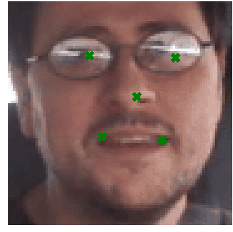
for irow in range(x_test.shape[0]):
img = x_test[irow]
ys = y_pred[irow]
fig = plt.figure(figsize=(10,10))
ax = fig.add_subplot(1,1,1)
ax.axis("off")
ax.imshow(img/255.0)
for x, y in zip(ys[0::2],ys[1::2]):
ax.scatter(x,y,c="green",s=500,marker="X")
plt.savefig(dir_image + "/fig{:04.0f}.png".format(irow),
bbox_inches='tight',pad_inches=0)
create_gif("driver_data_augmentation",dir_image,duration=0.5)
plt.close('all')