In this blog post, I will use np.fft.fft2 to experiment low pass filters and high pass filters.
**Low Pass Filtering** A low pass filter is the basis for most smoothing methods. An image is smoothed by decreasing the disparity between pixel values by averaging nearby pixels (see Smoothing an Image for more information).
**High Pass Filtering** A high pass filter is the basis for most sharpening methods. An image is sharpened when contrast is enhanced between adjoining areas with little variation in brightness or darkness (see Sharpening an Image for more detailed information).
Read an example image. Beautiful picture of Pumori from Kala Patthar.
In [1]:
import matplotlib.pyplot as plt
import numpy as np
img = plt.imread("GOPR0864.JPG")/float(2**8)
plt.imshow(img)
plt.show()
Before performing FFT on this beautiful image, I will create a draw_circle function that I will later use to trim the Frequency array generated by np.fft.fft2.
In [2]:
shape = img.shape[:2]

def draw_cicle(shape,diamiter):
    '''
    Input:
    shape    : tuple (height, width)
    diameter : scalar

    Output:
    np.array of shape  that says True within a circle with diamiter =  around center
    '''
    assert len(shape) == 2
    TF = np.zeros(shape,dtype=np.bool)
    center = np.array(TF.shape)/2.0

    for iy in range(shape[0]):
        for ix in range(shape[1]):
            TF[iy,ix] = (iy- center[0])**2 + (ix - center[1])**2 < diamiter **2
    return(TF)


TFcircleIN   = draw_cicle(shape=img.shape[:2],diamiter=50)
TFcircleOUT  = ~TFcircleIN

fig = plt.figure(figsize=(30,10))
ax  = fig.add_subplot(1,2,1)
im  = ax.imshow(TFcircleIN,cmap="gray")
plt.colorbar(im)
ax  = fig.add_subplot(1,2,2)
im  = ax.imshow(TFcircleOUT,cmap="gray")
plt.colorbar(im)
plt.show()

OK. Now I will perform FFT on every channel.
In [3]:
fft_img = np.zeros_like(img,dtype=complex)
for ichannel in range(fft_img.shape[2]):
    fft_img[:,:,ichannel] = np.fft.fftshift(np.fft.fft2(img[:,:,ichannel]))
From the FFT filter, I will create low pass filter, that only keeps low frequency FFT filter, and high pass filter, that only keeps high frequency FFT filter.
In [4]:
def filter_circle(TFcircleIN,fft_img_channel):
    temp = np.zeros(fft_img_channel.shape[:2],dtype=complex)
    temp[TFcircleIN] = fft_img_channel[TFcircleIN]
    return(temp)

fft_img_filtered_IN = []
fft_img_filtered_OUT = []
## for each channel, pass filter
for ichannel in range(fft_img.shape[2]):
    fft_img_channel  = fft_img[:,:,ichannel]
    ## circle IN
    temp = filter_circle(TFcircleIN,fft_img_channel)
    fft_img_filtered_IN.append(temp)
    ## circle OUT
    temp = filter_circle(TFcircleOUT,fft_img_channel)
    fft_img_filtered_OUT.append(temp)

fft_img_filtered_IN = np.array(fft_img_filtered_IN)
fft_img_filtered_IN = np.transpose(fft_img_filtered_IN,(1,2,0))
fft_img_filtered_OUT = np.array(fft_img_filtered_OUT)
fft_img_filtered_OUT = np.transpose(fft_img_filtered_OUT,(1,2,0))
In [5]:
abs_fft_img              = np.abs(fft_img)
abs_fft_img_filtered_IN  = np.abs(fft_img_filtered_IN)
abs_fft_img_filtered_OUT = np.abs(fft_img_filtered_OUT)
Visualize FFT filter, low pass filter and high pass filter.
In [6]:
def imshow_fft(absfft):
    magnitude_spectrum = 20*np.log(absfft)
    return(ax.imshow(magnitude_spectrum,cmap="gray"))

fig, axs = plt.subplots(nrows=3,ncols=3,figsize=(15,10))
fontsize = 15
for ichannel, color in enumerate(["R","G","B"]):
    ax = axs[0,ichannel]
    ax.set_title(color)
    im = imshow_fft(abs_fft_img[:,:,ichannel])
    ax.axis("off")
    if ichannel == 0:
        ax.set_ylabel("original DFT",fontsize=fontsize)
    fig.colorbar(im,ax=ax)


    ax = axs[1,ichannel]
    im = imshow_fft(abs_fft_img_filtered_IN[:,:,ichannel])
    ax.axis("off")
    if ichannel == 0:
        ax.set_ylabel("DFT + low pass filter",fontsize=fontsize)
    fig.colorbar(im,ax=ax)

    ax = axs[2,ichannel]
    im = imshow_fft(abs_fft_img_filtered_OUT[:,:,ichannel])
    ax.axis("off")
    if ichannel == 0:
        ax.set_ylabel("DFT + high pass filter",fontsize=fontsize)
    fig.colorbar(im,ax=ax)

plt.show()

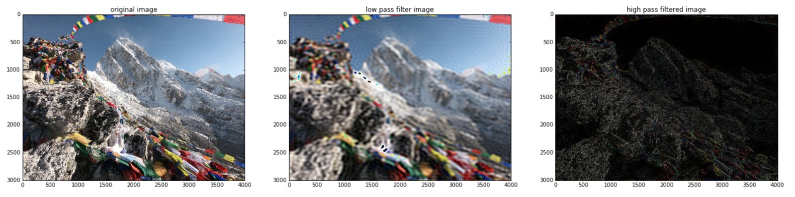
Finally, filter the original image and inverse-FFT the image
- Low Pass Filtering blurs the image.
- High Pass Filtering is an edge detection operation.
This also shows that most of the image data is present in the Low frequency region of the spectrum.
In [7]:
def inv_FFT_all_channel(fft_img):
    img_reco = []
    for ichannel in range(fft_img.shape[2]):
        img_reco.append(np.fft.ifft2(np.fft.ifftshift(fft_img[:,:,ichannel])))
    img_reco = np.array(img_reco)
    img_reco = np.transpose(img_reco,(1,2,0))
    return(img_reco)


img_reco              = inv_FFT_all_channel(fft_img)
img_reco_filtered_IN  = inv_FFT_all_channel(fft_img_filtered_IN)
img_reco_filtered_OUT = inv_FFT_all_channel(fft_img_filtered_OUT)

fig = plt.figure(figsize=(25,18))
ax  = fig.add_subplot(1,3,1)
ax.imshow(np.abs(img_reco))
ax.set_title("original image")

ax  = fig.add_subplot(1,3,2)
ax.imshow(np.abs(img_reco_filtered_IN))
ax.set_title("low pass filter image")


ax  = fig.add_subplot(1,3,3)
ax.imshow(np.abs(img_reco_filtered_OUT))
ax.set_title("high pass filtered image")
plt.show()
