Yumi's Blog

My first GAN using CelebA data

gif Everyone has been lately talking about Generative Adversarial Networks, or more famously known as GAN. My colleagues, interview candidates, my manager, conferences literally EVERYONE. It seems like the GANs becomes required knowledge for data scientists in bay area. It also seems that GANs are cool: GANs can generate new celebility face images, generate creative arts or generate the next frame of the video images. AI can think by itself with the power of GAN.

In this blog I will learn what's so great about GAN. The gif above is the outputed images from my first GAN. The reproduced images are blurr and seem to need more training; I only trained my GAN for about 1 hour. Nevertheless, this is a good start.

My focus in this blog will be on its simple implementation rather than its theoretical degails. I will use famous and popular celebA data to train GANs, and generate celebrity face images.

I got lots of good idea about its simple implemenation from GAN: A Beginner’s Guide to Generative Adversarial Networks so I highly recommend you to read this great blog first.

Reference

In [1]:
## load modules
import matplotlib.pyplot as plt
import os, time  
import numpy as np 
from keras.preprocessing.image import load_img
from keras.preprocessing.image import img_to_array

import tensorflow as tf
from keras.backend.tensorflow_backend import set_session


os.environ["CUDA_DEVICE_ORDER"] = "PCI_BUS_ID" 
config = tf.ConfigProto()
config.gpu_options.per_process_gpu_memory_fraction = 0.95
config.gpu_options.visible_device_list = "1" 
set_session(tf.Session(config=config))   
/home/bur2pal/anaconda2/lib/python2.7/site-packages/h5py/__init__.py:36: FutureWarning: Conversion of the second argument of issubdtype from `float` to `np.floating` is deprecated. In future, it will be treated as `np.float64 == np.dtype(float).type`.
  from ._conv import register_converters as _register_converters
Using TensorFlow backend.

Load celebA data.

As my previous post shows, celebA contains over 202,599 images. I will use 200,000 images to train GANs. The original image is of the shape (218, 178, 3). All images are resized to smaller shape for the sake of easier computation.

I am shrinking the image size pretty small here because otherwise, GAN requires lots of computation time.

In [2]:
dir_data      = "data/img_align_celeba/"
Ntrain        = 200000 
Ntest         = 100
nm_imgs       = np.sort(os.listdir(dir_data))
## name of the jpg files for training set
nm_imgs_train = nm_imgs[:Ntrain]
## name of the jpg files for the testing data
nm_imgs_test  = nm_imgs[Ntrain:Ntrain + Ntest]
img_shape     = (32, 32, 3)

def get_npdata(nm_imgs_train):
    X_train = []
    for i, myid in enumerate(nm_imgs_train):
        image = load_img(dir_data + "/" + myid,
                         target_size=img_shape[:2])
        image = img_to_array(image)/255.0
        X_train.append(image)
    X_train = np.array(X_train)
    return(X_train)

X_train = get_npdata(nm_imgs_train)
print("X_train.shape = {}".format(X_train.shape))

X_test  = get_npdata(nm_imgs_test)
print("X_test.shape = {}".format(X_test.shape))
X_train.shape = (200000, 32, 32, 3)
X_test.shape = (100, 32, 32, 3)

Plot the resized input images

I hope that our generators can generate images similar to these!

In [3]:
fig = plt.figure(figsize=(30,10))
nplot = 7
for count in range(1,nplot):
    ax = fig.add_subplot(1,nplot,count)
    ax.imshow(X_train[count])
plt.show()

Define GAN

GAN contains two networks which has two competing objectives:

  • Generator: the generator generates new data instances that are "similar" to the training data, in our case celebA images. Generator takes random latent vector and output a "fake" image of the same size as our reshaped celebA image.

  • Discriminator: the discriminator evaluate the authenticity of provided images; it classifies the images from the generator and the original image. Discriminator takes true of fake images and output the probability estimate ranging between 0 and 1.

\begin{array}{rcll} \textrm{Generator(latent)} &\rightarrow& \textrm{image}\\ \textrm{Discriminator(image)}&\rightarrow& \textrm{0 (fake) /1 (true)} \end{array}

Define generator

In [4]:
import numpy as np
from keras import layers, models
from keras.optimizers import Adam

## optimizer
#optimizer = Adam(0.0002, 0.5)
optimizer = Adam(0.00007, 0.5)

def build_generator(img_shape, noise_shape = (100,)):
    '''
    noise_shape : the dimension of the input vector for the generator
    img_shape   : the dimension of the output
    '''
    ## latent variable as input
    input_noise = layers.Input(shape=noise_shape) 
    d = layers.Dense(1024, activation="relu")(input_noise) 
    d = layers.Dense(1024, activation="relu")(input_noise) 
    d = layers.Dense(128*8*8, activation="relu")(d)
    d = layers.Reshape((8,8,128))(d)
    
    d = layers.Conv2DTranspose(128, kernel_size=(2,2) ,  strides=(2,2) , use_bias=False)(d)
    d = layers.Conv2D( 64  , ( 1 , 1 ) , activation='relu' , padding='same', name="block_4")(d) ## 16,16


    d = layers.Conv2DTranspose(32, kernel_size=(2,2) ,  strides=(2,2) , use_bias=False)(d)
    d = layers.Conv2D( 64  , ( 1 , 1 ) , activation='relu' , padding='same', name="block_5")(d) ## 32,32
    
    if img_shape[0] == 64:
        d = layers.Conv2DTranspose(32, kernel_size=(2,2) ,  strides=(2,2) , use_bias=False)(d)
        d = layers.Conv2D( 64  , ( 1 , 1 ) , activation='relu' , padding='same', name="block_6")(d) ## 64,64
    
    img = layers.Conv2D( 3 , ( 1 , 1 ) , activation='sigmoid' , padding='same', name="final_block")(d) ## 32, 32
    model = models.Model(input_noise, img)
    model.summary() 
    return(model)

## Set the dimension of latent variables to be 100
noise_shape = (100,)

generator = build_generator(img_shape, noise_shape = noise_shape)

generator.compile(loss='binary_crossentropy', optimizer=optimizer)
_________________________________________________________________
Layer (type)                 Output Shape              Param #   
=================================================================
input_1 (InputLayer)         (None, 100)               0         
_________________________________________________________________
dense_2 (Dense)              (None, 1024)              103424    
_________________________________________________________________
dense_3 (Dense)              (None, 8192)              8396800   
_________________________________________________________________
reshape_1 (Reshape)          (None, 8, 8, 128)         0         
_________________________________________________________________
conv2d_transpose_1 (Conv2DTr (None, 16, 16, 128)       65536     
_________________________________________________________________
block_4 (Conv2D)             (None, 16, 16, 64)        8256      
_________________________________________________________________
conv2d_transpose_2 (Conv2DTr (None, 32, 32, 32)        8192      
_________________________________________________________________
block_5 (Conv2D)             (None, 32, 32, 64)        2112      
_________________________________________________________________
final_block (Conv2D)         (None, 32, 32, 3)         195       
=================================================================
Total params: 8,584,515
Trainable params: 8,584,515
Non-trainable params: 0
_________________________________________________________________

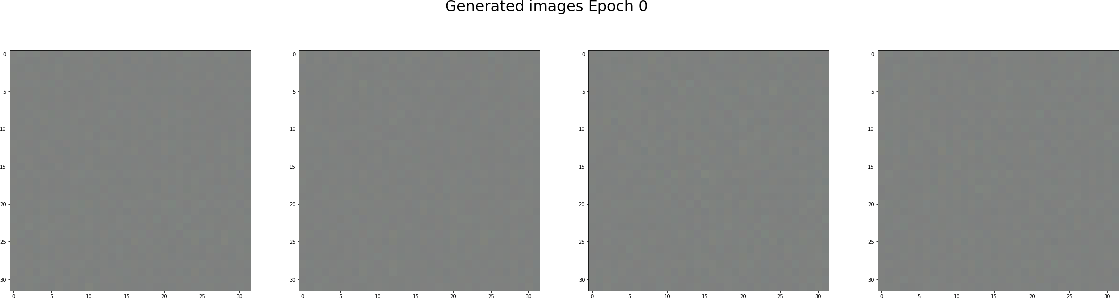
Take a look at the generatied images BEFORE any training.

As expectedly, the image is nothing like celebA. Our generator knows nothing about it and it outputs some random noise in a weak attempt to trick the discriminator. Let's see how much generator can learn from the celebA training data to generate "fake celebA images"!

In [5]:
def get_noise(nsample=1, nlatent_dim=100):
    noise = np.random.normal(0, 1, (nsample,nlatent_dim))
    return(noise)

def plot_generated_images(noise,path_save=None,titleadd=""):
    imgs = generator.predict(noise)
    fig = plt.figure(figsize=(40,10))
    for i, img in enumerate(imgs):
        ax = fig.add_subplot(1,nsample,i+1)
        ax.imshow(img)
    fig.suptitle("Generated images "+titleadd,fontsize=30)
    
    if path_save is not None:
        plt.savefig(path_save,
                    bbox_inches='tight',
                    pad_inches=0)
        plt.close()
    else:
        plt.show()

nsample = 4
noise = get_noise(nsample=nsample, nlatent_dim=noise_shape[0])
plot_generated_images(noise)

Define discriminator

In [6]:
def build_discriminator(img_shape,noutput=1):
    input_img = layers.Input(shape=img_shape)
    
    x = layers.Conv2D(32, (3, 3), activation='relu', padding='same', name='block1_conv1')(input_img)
    x = layers.Conv2D(32, (3, 3), activation='relu', padding='same', name='block1_conv2')(x)
    x = layers.MaxPooling2D((2, 2), strides=(2, 2), name='block1_pool')(x)
    
    x = layers.Conv2D(64, (3, 3), activation='relu', padding='same', name='block2_conv1')(x)
    x = layers.Conv2D(64, (3, 3), activation='relu', padding='same', name='block2_conv2')(x)
    x = layers.MaxPooling2D((2, 2), strides=(2, 2), name='block2_pool')(x)
    
    x = layers.Conv2D(128, (3, 3), activation='relu', padding='same', name='block4_conv1')(x)
    x = layers.Conv2D(128, (3, 3), activation='relu', padding='same', name='block4_conv2')(x)
    x = layers.MaxPooling2D((2, 2), strides=(1, 1), name='block4_pool')(x)

    
    x         = layers.Flatten()(x)
    x         = layers.Dense(1024,      activation="relu")(x)
    out       = layers.Dense(noutput,   activation='sigmoid')(x)
    model     = models.Model(input_img, out)
    
    return model

discriminator  = build_discriminator(img_shape)
discriminator.compile(loss      = 'binary_crossentropy', 
                      optimizer = optimizer,
                      metrics   = ['accuracy'])

discriminator.summary()
_________________________________________________________________
Layer (type)                 Output Shape              Param #   
=================================================================
input_2 (InputLayer)         (None, 32, 32, 3)         0         
_________________________________________________________________
block1_conv1 (Conv2D)        (None, 32, 32, 32)        896       
_________________________________________________________________
block1_conv2 (Conv2D)        (None, 32, 32, 32)        9248      
_________________________________________________________________
block1_pool (MaxPooling2D)   (None, 16, 16, 32)        0         
_________________________________________________________________
block2_conv1 (Conv2D)        (None, 16, 16, 64)        18496     
_________________________________________________________________
block2_conv2 (Conv2D)        (None, 16, 16, 64)        36928     
_________________________________________________________________
block2_pool (MaxPooling2D)   (None, 8, 8, 64)          0         
_________________________________________________________________
block4_conv1 (Conv2D)        (None, 8, 8, 128)         73856     
_________________________________________________________________
block4_conv2 (Conv2D)        (None, 8, 8, 128)         147584    
_________________________________________________________________
block4_pool (MaxPooling2D)   (None, 7, 7, 128)         0         
_________________________________________________________________
flatten_1 (Flatten)          (None, 6272)              0         
_________________________________________________________________
dense_4 (Dense)              (None, 1024)              6423552   
_________________________________________________________________
dense_5 (Dense)              (None, 1)                 1025      
=================================================================
Total params: 6,711,585
Trainable params: 6,711,585
Non-trainable params: 0
_________________________________________________________________

Combined model

In 32×32 8-bit RGB images, there are $2^{3x8x32x32}=2^{24576}$ possible arrangements of the pixel values in those images. The number of parameters of Generator and Dicriminator are together much less than this number.

  • noise -> generator -> discriminator

This combined model will share the same weights as discriminator and generator.

In [7]:
z = layers.Input(shape=noise_shape)
img = generator(z)

# For the combined model we will only train the generator
discriminator.trainable = False

# The valid takes generated images as input and determines validity
valid = discriminator(img)

# The combined model  (stacked generator and discriminator) takes
# noise as input => generates images => determines validity 
combined = models.Model(z, valid)
combined.compile(loss='binary_crossentropy', optimizer=optimizer)
combined.summary()
_________________________________________________________________
Layer (type)                 Output Shape              Param #   
=================================================================
input_3 (InputLayer)         (None, 100)               0         
_________________________________________________________________
model_1 (Model)              (None, 32, 32, 3)         8584515   
_________________________________________________________________
model_2 (Model)              (None, 1)                 6711585   
=================================================================
Total params: 15,296,100
Trainable params: 8,584,515
Non-trainable params: 6,711,585
_________________________________________________________________

Training

When you train the discriminator, hold the generator values constant; and when you train the generator, hold the discriminator constant.

In [8]:
def train(models, X_train, noise_plot, dir_result="/result/", epochs=10000, batch_size=128):
        '''
        models     : tuple containins three tensors, (combined, discriminator, generator)
        X_train    : np.array containing images (Nsample, height, width, Nchannels)
        noise_plot : np.array of size (Nrandom_sample_to_plot, hidden unit length)
        dir_result : the location where the generated plots for noise_plot are saved 
        
        '''
        combined, discriminator, generator = models
        nlatent_dim = noise_plot.shape[1]
        half_batch  = int(batch_size / 2)
        history = []
        for epoch in range(epochs):

            # ---------------------
            #  Train Discriminator
            # ---------------------

            # Select a random half batch of images
            idx = np.random.randint(0, X_train.shape[0], half_batch)
            imgs = X_train[idx]
            noise = get_noise(half_batch, nlatent_dim)

            # Generate a half batch of new images
            gen_imgs = generator.predict(noise)

            
            # Train the discriminator q: better to mix them together?
            d_loss_real = discriminator.train_on_batch(imgs, np.ones((half_batch, 1)))
            d_loss_fake = discriminator.train_on_batch(gen_imgs, np.zeros((half_batch, 1)))
            d_loss = 0.5 * np.add(d_loss_real, d_loss_fake)


            # ---------------------
            #  Train Generator
            # ---------------------

            noise = get_noise(batch_size, nlatent_dim)

            # The generator wants the discriminator to label the generated samples
            # as valid (ones)
            valid_y = (np.array([1] * batch_size)).reshape(batch_size,1)
            
            # Train the generator
            g_loss = combined.train_on_batch(noise, valid_y)

            history.append({"D":d_loss[0],"G":g_loss})
            
            if epoch % 100 == 0:
                # Plot the progress
                print ("Epoch {:05.0f} [D loss: {:4.3f}, acc.: {:05.1f}%] [G loss: {:4.3f}]".format(
                    epoch, d_loss[0], 100*d_loss[1], g_loss))
            if epoch % int(epochs/100) == 0:
                plot_generated_images(noise_plot,
                                      path_save=dir_result+"/image_{:05.0f}.png".format(epoch),
                                      titleadd="Epoch {}".format(epoch))
            if epoch % 1000 == 0:
                plot_generated_images(noise_plot,
                                      titleadd="Epoch {}".format(epoch))
                        
        return(history)

dir_result="./result_GAN/"

try:
    os.mkdir(dir_result)
except:
    pass
    
start_time = time.time()

_models = combined, discriminator, generator          

history = train(_models, X_train, noise, dir_result=dir_result,epochs=20000, batch_size=128*8)
end_time = time.time()
print("-"*10)
print("Time took: {:4.2f} min".format((end_time - start_time)/60))
/home/bur2pal/Modules/keras/keras/engine/training.py:973: UserWarning: Discrepancy between trainable weights and collected trainable weights, did you set `model.trainable` without calling `model.compile` after ?
  'Discrepancy between trainable weights and collected trainable'
Epoch 00000 [D loss: 0.732, acc.: 038.4%] [G loss: 0.648]
Epoch 00100 [D loss: 0.098, acc.: 098.2%] [G loss: 3.399]
Epoch 00200 [D loss: 0.272, acc.: 089.1%] [G loss: 2.390]
Epoch 00300 [D loss: 0.271, acc.: 088.7%] [G loss: 2.464]
Epoch 00400 [D loss: 0.282, acc.: 089.1%] [G loss: 2.234]
Epoch 00500 [D loss: 0.185, acc.: 093.0%] [G loss: 2.780]
Epoch 00600 [D loss: 0.213, acc.: 094.7%] [G loss: 3.204]
Epoch 00700 [D loss: 0.161, acc.: 095.7%] [G loss: 3.229]
Epoch 00800 [D loss: 0.168, acc.: 095.3%] [G loss: 4.831]
Epoch 00900 [D loss: 0.189, acc.: 093.6%] [G loss: 2.705]
Epoch 01000 [D loss: 0.295, acc.: 089.1%] [G loss: 2.081]
Epoch 01100 [D loss: 0.232, acc.: 092.6%] [G loss: 2.619]
Epoch 01200 [D loss: 0.158, acc.: 093.7%] [G loss: 3.485]
Epoch 01300 [D loss: 0.284, acc.: 089.9%] [G loss: 3.901]
Epoch 01400 [D loss: 0.129, acc.: 095.8%] [G loss: 3.299]
Epoch 01500 [D loss: 0.345, acc.: 084.4%] [G loss: 3.596]
Epoch 01600 [D loss: 0.346, acc.: 086.7%] [G loss: 2.375]
Epoch 01700 [D loss: 0.151, acc.: 095.8%] [G loss: 3.398]
Epoch 01800 [D loss: 0.169, acc.: 093.9%] [G loss: 3.201]
Epoch 01900 [D loss: 0.176, acc.: 093.9%] [G loss: 2.934]
Epoch 02000 [D loss: 0.169, acc.: 094.4%] [G loss: 3.022]
Epoch 02100 [D loss: 0.170, acc.: 094.0%] [G loss: 3.029]
Epoch 02200 [D loss: 0.346, acc.: 085.3%] [G loss: 2.539]
Epoch 02300 [D loss: 0.308, acc.: 087.7%] [G loss: 2.795]
Epoch 02400 [D loss: 0.372, acc.: 084.0%] [G loss: 2.897]
Epoch 02500 [D loss: 0.303, acc.: 088.2%] [G loss: 2.476]
Epoch 02600 [D loss: 0.331, acc.: 086.3%] [G loss: 2.522]
Epoch 02700 [D loss: 0.430, acc.: 081.0%] [G loss: 2.143]
Epoch 02800 [D loss: 0.409, acc.: 081.1%] [G loss: 2.220]
Epoch 02900 [D loss: 0.440, acc.: 079.1%] [G loss: 2.105]
Epoch 03000 [D loss: 0.419, acc.: 081.3%] [G loss: 2.262]
Epoch 03100 [D loss: 0.487, acc.: 078.3%] [G loss: 1.833]
Epoch 03200 [D loss: 0.497, acc.: 075.9%] [G loss: 1.826]
Epoch 03300 [D loss: 0.433, acc.: 081.2%] [G loss: 1.919]
Epoch 03400 [D loss: 0.371, acc.: 085.0%] [G loss: 2.259]
Epoch 03500 [D loss: 0.453, acc.: 078.8%] [G loss: 2.058]
Epoch 03600 [D loss: 0.471, acc.: 078.8%] [G loss: 1.663]
Epoch 03700 [D loss: 0.439, acc.: 080.0%] [G loss: 1.733]
Epoch 03800 [D loss: 0.499, acc.: 077.1%] [G loss: 1.587]
Epoch 03900 [D loss: 0.452, acc.: 079.3%] [G loss: 1.616]
Epoch 04000 [D loss: 0.502, acc.: 076.2%] [G loss: 1.670]
Epoch 04100 [D loss: 0.524, acc.: 074.2%] [G loss: 1.557]
Epoch 04200 [D loss: 0.468, acc.: 078.7%] [G loss: 1.523]
Epoch 04300 [D loss: 0.525, acc.: 072.5%] [G loss: 1.548]
Epoch 04400 [D loss: 0.502, acc.: 075.5%] [G loss: 1.492]
Epoch 04500 [D loss: 0.473, acc.: 077.1%] [G loss: 1.679]
Epoch 04600 [D loss: 0.478, acc.: 077.9%] [G loss: 1.628]
Epoch 04700 [D loss: 0.548, acc.: 072.3%] [G loss: 1.359]
Epoch 04800 [D loss: 0.538, acc.: 072.9%] [G loss: 1.341]
Epoch 04900 [D loss: 0.519, acc.: 075.3%] [G loss: 1.320]
Epoch 05000 [D loss: 0.452, acc.: 079.0%] [G loss: 1.521]
Epoch 05100 [D loss: 0.497, acc.: 075.9%] [G loss: 1.427]
Epoch 05200 [D loss: 0.497, acc.: 075.6%] [G loss: 1.370]
Epoch 05300 [D loss: 0.481, acc.: 077.1%] [G loss: 1.441]
Epoch 05400 [D loss: 0.514, acc.: 075.5%] [G loss: 1.377]
Epoch 05500 [D loss: 0.450, acc.: 080.4%] [G loss: 1.443]
Epoch 05600 [D loss: 0.489, acc.: 076.1%] [G loss: 1.415]
Epoch 05700 [D loss: 0.491, acc.: 075.9%] [G loss: 1.376]
Epoch 05800 [D loss: 0.479, acc.: 077.1%] [G loss: 1.531]
Epoch 05900 [D loss: 0.503, acc.: 076.0%] [G loss: 1.383]
Epoch 06000 [D loss: 0.476, acc.: 077.4%] [G loss: 1.395]
Epoch 06100 [D loss: 0.476, acc.: 078.0%] [G loss: 1.432]
Epoch 06200 [D loss: 0.505, acc.: 075.1%] [G loss: 1.374]
Epoch 06300 [D loss: 0.489, acc.: 076.0%] [G loss: 1.416]
Epoch 06400 [D loss: 0.484, acc.: 076.0%] [G loss: 1.459]
Epoch 06500 [D loss: 0.472, acc.: 077.5%] [G loss: 1.460]
Epoch 06600 [D loss: 0.554, acc.: 071.0%] [G loss: 1.387]
Epoch 06700 [D loss: 0.473, acc.: 077.3%] [G loss: 1.447]
Epoch 06800 [D loss: 0.529, acc.: 073.0%] [G loss: 1.378]
Epoch 06900 [D loss: 0.524, acc.: 073.2%] [G loss: 1.350]
Epoch 07000 [D loss: 0.495, acc.: 075.5%] [G loss: 1.321]
Epoch 07100 [D loss: 0.514, acc.: 074.4%] [G loss: 1.349]
Epoch 07200 [D loss: 0.468, acc.: 078.7%] [G loss: 1.469]
Epoch 07300 [D loss: 0.474, acc.: 076.4%] [G loss: 1.497]
Epoch 07400 [D loss: 0.442, acc.: 080.6%] [G loss: 1.465]
Epoch 07500 [D loss: 0.478, acc.: 076.6%] [G loss: 1.431]
Epoch 07600 [D loss: 0.504, acc.: 074.8%] [G loss: 1.375]
Epoch 07700 [D loss: 0.514, acc.: 073.3%] [G loss: 1.393]
Epoch 07800 [D loss: 0.511, acc.: 074.2%] [G loss: 1.376]
Epoch 07900 [D loss: 0.510, acc.: 075.4%] [G loss: 1.378]
Epoch 08000 [D loss: 0.508, acc.: 075.1%] [G loss: 1.388]
Epoch 08100 [D loss: 0.498, acc.: 075.5%] [G loss: 1.425]
Epoch 08200 [D loss: 0.477, acc.: 077.1%] [G loss: 1.425]
Epoch 08300 [D loss: 0.491, acc.: 077.0%] [G loss: 1.364]
Epoch 08400 [D loss: 0.521, acc.: 073.5%] [G loss: 1.331]
Epoch 08500 [D loss: 0.455, acc.: 079.2%] [G loss: 1.392]
Epoch 08600 [D loss: 0.496, acc.: 075.4%] [G loss: 1.421]
Epoch 08700 [D loss: 0.473, acc.: 077.0%] [G loss: 1.396]
Epoch 08800 [D loss: 0.494, acc.: 075.5%] [G loss: 1.427]
Epoch 08900 [D loss: 0.508, acc.: 073.9%] [G loss: 1.384]
Epoch 09000 [D loss: 0.502, acc.: 075.1%] [G loss: 1.369]
Epoch 09100 [D loss: 0.460, acc.: 077.9%] [G loss: 1.337]
Epoch 09200 [D loss: 0.492, acc.: 075.8%] [G loss: 1.401]
Epoch 09300 [D loss: 0.465, acc.: 078.1%] [G loss: 1.371]
Epoch 09400 [D loss: 0.506, acc.: 075.4%] [G loss: 1.365]
Epoch 09500 [D loss: 0.472, acc.: 077.9%] [G loss: 1.315]
Epoch 09600 [D loss: 0.453, acc.: 079.0%] [G loss: 1.366]
Epoch 09700 [D loss: 0.482, acc.: 075.9%] [G loss: 1.353]
Epoch 09800 [D loss: 0.505, acc.: 075.0%] [G loss: 1.372]
Epoch 09900 [D loss: 0.511, acc.: 074.9%] [G loss: 1.356]
Epoch 10000 [D loss: 0.477, acc.: 077.0%] [G loss: 1.396]
Epoch 10100 [D loss: 0.476, acc.: 077.8%] [G loss: 1.324]
Epoch 10200 [D loss: 0.475, acc.: 077.0%] [G loss: 1.377]
Epoch 10300 [D loss: 0.507, acc.: 074.0%] [G loss: 1.361]
Epoch 10400 [D loss: 0.466, acc.: 076.4%] [G loss: 1.414]
Epoch 10500 [D loss: 0.492, acc.: 074.1%] [G loss: 1.365]
Epoch 10600 [D loss: 0.469, acc.: 078.6%] [G loss: 1.340]
Epoch 10700 [D loss: 0.474, acc.: 077.2%] [G loss: 1.371]
Epoch 10800 [D loss: 0.492, acc.: 074.4%] [G loss: 1.348]
Epoch 10900 [D loss: 0.471, acc.: 077.3%] [G loss: 1.349]
Epoch 11000 [D loss: 0.472, acc.: 077.8%] [G loss: 1.342]
Epoch 11100 [D loss: 0.447, acc.: 080.1%] [G loss: 1.408]
Epoch 11200 [D loss: 0.473, acc.: 076.6%] [G loss: 1.367]
Epoch 11300 [D loss: 0.465, acc.: 078.5%] [G loss: 1.395]
Epoch 11400 [D loss: 0.479, acc.: 077.2%] [G loss: 1.352]
Epoch 11500 [D loss: 0.509, acc.: 074.4%] [G loss: 1.306]
Epoch 11600 [D loss: 0.490, acc.: 074.0%] [G loss: 1.323]
Epoch 11700 [D loss: 0.490, acc.: 075.4%] [G loss: 1.321]
Epoch 11800 [D loss: 0.506, acc.: 074.3%] [G loss: 1.315]
Epoch 11900 [D loss: 0.497, acc.: 075.6%] [G loss: 1.325]
Epoch 12000 [D loss: 0.491, acc.: 075.8%] [G loss: 1.317]
Epoch 12100 [D loss: 0.501, acc.: 074.9%] [G loss: 1.371]
Epoch 12200 [D loss: 0.488, acc.: 074.9%] [G loss: 1.391]
Epoch 12300 [D loss: 0.527, acc.: 073.4%] [G loss: 1.332]
Epoch 12400 [D loss: 0.486, acc.: 074.8%] [G loss: 1.350]
Epoch 12500 [D loss: 0.482, acc.: 077.0%] [G loss: 1.321]
Epoch 12600 [D loss: 0.511, acc.: 074.4%] [G loss: 1.325]
Epoch 12700 [D loss: 0.507, acc.: 074.1%] [G loss: 1.329]
Epoch 12800 [D loss: 0.501, acc.: 074.3%] [G loss: 1.338]
Epoch 12900 [D loss: 0.482, acc.: 078.2%] [G loss: 1.367]
Epoch 13000 [D loss: 0.488, acc.: 076.9%] [G loss: 1.386]
Epoch 13100 [D loss: 0.505, acc.: 074.5%] [G loss: 1.335]
Epoch 13200 [D loss: 0.509, acc.: 074.1%] [G loss: 1.318]
Epoch 13300 [D loss: 0.496, acc.: 075.2%] [G loss: 1.379]
Epoch 13400 [D loss: 0.475, acc.: 076.3%] [G loss: 1.392]
Epoch 13500 [D loss: 0.508, acc.: 073.6%] [G loss: 1.338]
Epoch 13600 [D loss: 0.461, acc.: 077.7%] [G loss: 1.342]
Epoch 13700 [D loss: 0.485, acc.: 075.8%] [G loss: 1.350]
Epoch 13800 [D loss: 0.462, acc.: 078.9%] [G loss: 1.358]
Epoch 13900 [D loss: 0.486, acc.: 076.2%] [G loss: 1.383]
Epoch 14000 [D loss: 0.475, acc.: 078.4%] [G loss: 1.410]
Epoch 14100 [D loss: 0.511, acc.: 075.0%] [G loss: 1.326]
Epoch 14200 [D loss: 0.487, acc.: 075.9%] [G loss: 1.301]
Epoch 14300 [D loss: 0.510, acc.: 074.2%] [G loss: 1.372]
Epoch 14400 [D loss: 0.510, acc.: 074.5%] [G loss: 1.395]
Epoch 14500 [D loss: 0.506, acc.: 073.2%] [G loss: 1.350]
Epoch 14600 [D loss: 0.478, acc.: 078.2%] [G loss: 1.402]
Epoch 14700 [D loss: 0.497, acc.: 075.6%] [G loss: 1.374]
Epoch 14800 [D loss: 0.468, acc.: 077.7%] [G loss: 1.382]
Epoch 14900 [D loss: 0.470, acc.: 077.2%] [G loss: 1.337]
Epoch 15000 [D loss: 0.475, acc.: 078.9%] [G loss: 1.326]
Epoch 15100 [D loss: 0.477, acc.: 076.4%] [G loss: 1.347]
Epoch 15200 [D loss: 0.463, acc.: 077.9%] [G loss: 1.386]
Epoch 15300 [D loss: 0.484, acc.: 076.3%] [G loss: 1.326]
Epoch 15400 [D loss: 0.494, acc.: 076.6%] [G loss: 1.282]
Epoch 15500 [D loss: 0.483, acc.: 077.0%] [G loss: 1.364]
Epoch 15600 [D loss: 0.502, acc.: 074.1%] [G loss: 1.387]
Epoch 15700 [D loss: 0.478, acc.: 076.7%] [G loss: 1.359]
Epoch 15800 [D loss: 0.489, acc.: 074.8%] [G loss: 1.339]
Epoch 15900 [D loss: 0.504, acc.: 074.8%] [G loss: 1.362]
Epoch 16000 [D loss: 0.480, acc.: 075.4%] [G loss: 1.354]
Epoch 16100 [D loss: 0.486, acc.: 075.5%] [G loss: 1.381]
Epoch 16200 [D loss: 0.491, acc.: 076.6%] [G loss: 1.374]
Epoch 16300 [D loss: 0.496, acc.: 074.2%] [G loss: 1.421]
Epoch 16400 [D loss: 0.468, acc.: 076.6%] [G loss: 1.416]
Epoch 16500 [D loss: 0.492, acc.: 076.2%] [G loss: 1.359]
Epoch 16600 [D loss: 0.500, acc.: 073.6%] [G loss: 1.341]
Epoch 16700 [D loss: 0.475, acc.: 076.4%] [G loss: 1.409]
Epoch 16800 [D loss: 0.476, acc.: 077.8%] [G loss: 1.377]
Epoch 16900 [D loss: 0.482, acc.: 075.7%] [G loss: 1.397]
Epoch 17000 [D loss: 0.465, acc.: 077.3%] [G loss: 1.371]
Epoch 17100 [D loss: 0.492, acc.: 074.9%] [G loss: 1.340]
Epoch 17200 [D loss: 0.486, acc.: 076.2%] [G loss: 1.383]
Epoch 17300 [D loss: 0.458, acc.: 078.1%] [G loss: 1.411]
Epoch 17400 [D loss: 0.476, acc.: 077.6%] [G loss: 1.413]
Epoch 17500 [D loss: 0.501, acc.: 074.5%] [G loss: 1.401]
Epoch 17600 [D loss: 0.500, acc.: 074.5%] [G loss: 1.396]
Epoch 17700 [D loss: 0.470, acc.: 076.1%] [G loss: 1.365]
Epoch 17800 [D loss: 0.489, acc.: 075.6%] [G loss: 1.415]
Epoch 17900 [D loss: 0.485, acc.: 076.1%] [G loss: 1.412]
Epoch 18000 [D loss: 0.478, acc.: 077.0%] [G loss: 1.437]
Epoch 18100 [D loss: 0.473, acc.: 077.3%] [G loss: 1.396]
Epoch 18200 [D loss: 0.436, acc.: 081.0%] [G loss: 1.382]
Epoch 18300 [D loss: 0.500, acc.: 074.9%] [G loss: 1.466]
Epoch 18400 [D loss: 0.485, acc.: 076.5%] [G loss: 1.415]
Epoch 18500 [D loss: 0.454, acc.: 078.9%] [G loss: 1.432]
Epoch 18600 [D loss: 0.484, acc.: 075.6%] [G loss: 1.444]
Epoch 18700 [D loss: 0.435, acc.: 079.7%] [G loss: 1.391]
Epoch 18800 [D loss: 0.481, acc.: 077.0%] [G loss: 1.427]
Epoch 18900 [D loss: 0.488, acc.: 076.4%] [G loss: 1.428]
Epoch 19000 [D loss: 0.466, acc.: 078.3%] [G loss: 1.380]
Epoch 19100 [D loss: 0.473, acc.: 075.8%] [G loss: 1.427]
Epoch 19200 [D loss: 0.462, acc.: 075.9%] [G loss: 1.478]
Epoch 19300 [D loss: 0.458, acc.: 078.0%] [G loss: 1.508]
Epoch 19400 [D loss: 0.483, acc.: 074.5%] [G loss: 1.402]
Epoch 19500 [D loss: 0.458, acc.: 076.9%] [G loss: 1.442]
Epoch 19600 [D loss: 0.477, acc.: 076.9%] [G loss: 1.392]
Epoch 19700 [D loss: 0.436, acc.: 080.2%] [G loss: 1.453]
Epoch 19800 [D loss: 0.469, acc.: 076.3%] [G loss: 1.426]
Epoch 19900 [D loss: 0.464, acc.: 077.6%] [G loss: 1.457]
----------
Time took: 76.88 min

Loss over epochs

Notice that the losses from dicriminator are not dicreasing over epochs, which makes sense because the discriminator's good classification performance is always challenged by the improved "fake images" from the generator.

In [9]:
import pandas as pd 
hist = pd.DataFrame(history)
plt.figure(figsize=(20,5))
for colnm in hist.columns:
    plt.plot(hist[colnm],label=colnm)
plt.legend()
plt.ylabel("loss")
plt.xlabel("epochs")
plt.show()

Finally create gif of the generated images at every few epochs

In [10]:
def makegif(dir_images):
    import imageio
    filenames = np.sort(os.listdir(dir_images))
    filenames = [ fnm for fnm in filenames if ".png" in fnm]

    with imageio.get_writer(dir_images + '/image.gif', mode='I') as writer:
        for filename in filenames:
            image = imageio.imread(dir_images + filename)
            writer.append_data(image)
            os.remove(dir_images + filename)
            
makegif(dir_result)

GAN Auto-Encoder

GAN can transform the latent variable to an image. What about the other way? Can I map an image to a latent variable? If we can do such mapping, I can do interesting things e.g., the average latent variable values of female images may be decoded into an average female images.

Photo Editing Generative Adversarial Networks Part 1 creates GAN-based encoder-decoder network: separately train an encoder while using generator as a fixed decoder. For the encoder network, I will use the discriminator with the number of output neurons in the last layer set to 100. This way, I can reversed the order of things in my GAN and created a GAN Auto-encoder.

In the encoder network, the trainable parameters are only set to the ones from the encoder.

In [11]:
img_in = layers.Input(shape=img_shape)

# discriminator with the final output layer = 100 network as encoder
discriminator_encoder = build_discriminator(img_shape,100)

# discriminator as encoder
encoder = discriminator_encoder(img_in)

# generator as decoder
generator.trainable = False
img_out = generator(encoder) 

encoder_decoder = models.Model(img_in,img_out)
encoder_decoder.compile(loss='mse', optimizer=optimizer)

encoder_decoder.summary()
_________________________________________________________________
Layer (type)                 Output Shape              Param #   
=================================================================
input_4 (InputLayer)         (None, 32, 32, 3)         0         
_________________________________________________________________
model_4 (Model)              (None, 100)               6813060   
_________________________________________________________________
model_1 (Model)              (None, 32, 32, 3)         8584515   
=================================================================
Total params: 15,397,575
Trainable params: 6,813,060
Non-trainable params: 8,584,515
_________________________________________________________________

Train encoders

In [12]:
start_time = time.time()
history_ed = encoder_decoder.fit(X_train,X_train,
                                 validation_data=(X_test,X_test),
                                 epochs=10,verbose=2)
end_time = time.time()
print("-"*10)
print("Time took: {:4.2f} min".format((end_time - start_time)/60))
Train on 200000 samples, validate on 100 samples
Epoch 1/10
 - 68s - loss: 0.0355 - val_loss: 0.0349
Epoch 2/10
 - 66s - loss: 0.0328 - val_loss: 0.0340
Epoch 3/10
 - 66s - loss: 0.0322 - val_loss: 0.0336
Epoch 4/10
 - 66s - loss: 0.0318 - val_loss: 0.0332
Epoch 5/10
 - 67s - loss: 0.0316 - val_loss: 0.0331
Epoch 6/10
 - 66s - loss: 0.0314 - val_loss: 0.0330
Epoch 7/10
 - 66s - loss: 0.0312 - val_loss: 0.0328
Epoch 8/10
 - 67s - loss: 0.0311 - val_loss: 0.0327
Epoch 9/10
 - 67s - loss: 0.0310 - val_loss: 0.0326
Epoch 10/10
 - 66s - loss: 0.0309 - val_loss: 0.0326
----------
Time took: 11.08 min

Loss over epochs

In [13]:
plt.figure(figsize=(10,5))
for colnm in history_ed.history.keys():
    plt.plot(history_ed.history[colnm],label=colnm)
plt.legend()
plt.show()

Check the model performance of the encoder-decoder network using testing data

In [14]:
# discriminator_encoder.compile(loss='mse', optimizer=optimizer)
X_pred = encoder_decoder.predict(X_test)
## z_pred = discriminator_encoder.predict(X_test)

Plot the original image and reproduced image using encoder

Some reproduced images are somewhat similar to the original images... But I clearly need more training.

In [15]:
Ntest = 10

for irow in range(Ntest):
    fig = plt.figure(figsize=(10,5))
    ax = fig.add_subplot(1,2,1)
    ax.imshow(X_test[irow])
    ax.set_title("original image")
    
    ax = fig.add_subplot(1,2,2)
    ax.imshow(X_pred[irow])
    ax.set_title("encoded image")
    
    plt.show()

Comments