In my previous blog, I reviewed PCA.
The Principal Component Analysis (PCA) techinique is often applied on sample dataframe of shape (Nsample, Nfeat).
In this blog, I will discuss how to obtain the PCA when the provided data is a two-dimensional heatmap.
The two-dimensional heatmap can be thought as a bivariate density on discretized constraint space.
It is discrete because the densiy values are evaluated only at pixcel grids,
and constraint because the grids are bounded.
Approach
In the previous blog, it was shown that the PCA only uses the sample variance as input and the original sample dataframe is not neccesary. Therefore, I will first obtain the estimate of the variance matrix from the provided heatmap, and then simply perform PCA on the estimated variance matrix.
import matplotlib.pyplot as plt
#img = load_img("plot_PCA_from_heatmap.png")

import numpy as np
Prepare Gaussian heatmap data
I will create a heatmap of size (width = 92, height = 86). The heatmap contains the bivariate Guassian density with correlation 0.4. Notice that the correlation is positive but the heatmap looks negatively correlated. But don't get misreaded. The origin of the imshow image is at the left top.
def biv_gaussian_k(x0,y0,sigma, width, height):
        """
        Create a heatmap of size (height, width) containing
        density values of bivariate gaussian centered at (x0, y0) and

        - Var(X)   = sigmax
        - Var(Y)   = sigmay
        - Cor(X,Y) = rho

        sigma = (sigmax, sigmay, rho)

        when sigmax = sigmay and rho = 0

        Note:
        This density does not have normalized constant
        """
        sigmax, sigmay, rho = sigma
        x = np.arange(0, width, 1, float) ## (width,)
        y = np.arange(0, height, 1, float)[:, np.newaxis] ## (height,1)
        term1 = -1/(2.*(1 - (rho**2)))

        term2 = (x - x0)**2 / (sigmax**2)
        term3 = (y - y0)**2 / (sigmay**2)
        term4 = -2.0*rho*(x - x0)*(y - y0)/(sigmax*sigmay)
        return np.exp(term1*( term2 + term3 + term4))

def biv_gaussian_constant(sigma):
        '''
        normalized constant for bivariate densiy with sigma
        the defenition of sigma is the same as the one from biv_gaussian_k
        '''
        sigmax, sigmay, rho = sigma
        const = 1/(2*np.pi*sigmax*sigmay*np.sqrt(1-(rho**2)))
        return(const)

# example
width, height = 92, 86
mx, my = 40,50
sigma  = (5,5.2,0.4)
arr = biv_gaussian_k(mx, my,
                     sigma,
                     width=width, height=height)
const = biv_gaussian_constant(sigma)
total_density = np.sum(arr*const)
plt.figure(figsize=(10,10))
plt.imshow(arr)
plt.title("Gaussian density (with normalized constant)= {:5.4f}".format(total_density))
plt.show()

Now I will shift the mean closer to the border. As the portion of density is outside of the image, the total sum of the provided densiy does not add up to 1.
mx, my = 90,50
arr = biv_gaussian_k(mx, my,
                     sigma,
                     width=width, height=height)
const = biv_gaussian_constant(sigma)
total_density = np.sum(arr*const)
plt.figure(figsize=(10,10))
plt.imshow(arr)
plt.title("Gaussian density (with normalized constant)= {:5.4f}".format(total_density))
plt.show()

Recover Gaussian density parameters from heatmap
In the PCA review section, we learned that the PCA only needs sample variance and not the sample dataframe. So I will present how to "estimate" the variance matrix using heatmap.
- Heatmap data -> Gaussian density
The following functions compute marginal mean and variance of heatmap.
def get_merginal_mean(arr,dim="x", meanNN_TF=False):
        '''
        E(x) = int x f(x) dx

        arr      : np.array containing 2-d heatmap, shape is (height, width)
        dim      : if "x", the marginal mean of X (width) is calcualted
                   if "y", the marginal mean of Y (height)is calcualted
        meanNN_TF: if False, the marginal mean is calculated using all the pixels.
                   if True, then the marginal mean is calculated using the neighboor of the high marginal density region.
                   The "neighboor" is calculated in two steps:
                   (1) order the intensity of the marginal density
                   in the decreasing manner,
                   (2) include the top densities until the corresponding pixel coordinate hits the pixel border.

        '''
        if dim == "x":
            axis = 0
        elif dim == "y":
            axis = 1
        mardens = arr.sum(axis=axis)
        asort   = np.argsort(mardens)[::-1]

        if meanNN_TF:
            Npixel = np.min(np.where((asort == 0) | (asort == (len(asort)-1) ))) + 1
        else:
            Npixel = -1
        mardens = mardens[asort][:Npixel]
        mardens /= np.sum(mardens) ## rescale so that marginal density adds up to 1

        xcoor   = asort[:Npixel]

        meanx   = np.sum((xcoor*mardens)[:Npixel])
        return(meanx)

def get_merginal_sd(arr,dim="x",verbose=False,meanNN_TF=False):
        '''
         E( (x - barx)**2 ) = int (x-barx)**2 f(x) dx

        arr     : np.array containing 2-d heatmap, shape is (height, width)
        dim     : if "x", the marginal mean of X (width) is calcualted
                  if "y", the marginal mean of Y (height)is calcualted
        meanNN_TF: if False, the marginal mean is calculated using all the pixels.
                   if True, then the marginal mean is calculated using the neighboor of the high marginal density region.
                   The "neighboor" is calculated in two steps:
                   (1) order the intensity of the marginal density
                   in the decreasing manner,
                   (2) include the top densities until the corresponding pixel coordinate hits the pixel border.
        '''
        if dim == "x":
            axis = 0
        elif dim == "y":
            axis = 1
        mardens = arr.sum(axis=axis)
        xcoor   = np.arange(len(mardens))

        meanx   = get_merginal_mean(arr, dim=dim, meanNN_TF=meanNN_TF)
        varx    = np.sqrt(np.sum((xcoor - meanx)**2*mardens))
        if verbose:
            print("{} total dens = {:4.3f}, mean = {:5.2f}".format(
                  dim,
                  np.sum(mardens),
                  meanx)
                 )
        return(varx)
def get_cov(arr,verbose=True,meanNN_TF=False):
        '''
         E( (x - barx)*(y - bary) ) = int (x-barx)*(y - bary) f(x,y) dxdy

        arr     : np.array containing 2-d heatmap, shape is (height, width)
        meanNN_TF: if False, the marginal mean is calculated using all the pixels.
                   if True, then the marginal mean is calculated using the neighboor of the high marginal density region.
                   The "neighboor" is calculated in two steps:
                   (1) order the intensity of the marginal density
                   in the decreasing manner,
                   (2) include the top densities until the corresponding pixel coordinate hits the pixel border.

                    recommended to set True to improve the variance estimate performance when not all the density is included in the heatmap image.

        '''

        ## prepare the storage space
        x_coor_mat = np.zeros_like(arr)
        for icol in range(x_coor_mat.shape[1]):
            x_coor_mat[:, icol] = icol

        y_coor_mat = np.zeros_like(arr)
        for irow in range(y_coor_mat.shape[0]):
            y_coor_mat[irow, :] = irow

        meanx   = get_merginal_mean(arr, dim = "x", meanNN_TF=meanNN_TF) ## scalar
        meany   = get_merginal_mean(arr, dim = "y", meanNN_TF=meanNN_TF) ## scalar

        cov     = np.sum((x_coor_mat - meanx)*(y_coor_mat - meany )*arr)

        return(cov)
Calculate the Gaussian parameters without normalization of heatmap
The plot below shows the heatmaps, its true Gaussian density parameter values, and their estimates.
Let $I(X,Y)$ be the intensity of the heatmap evaluated at $(X,Y)$, and let its marginal density be $I(X) = \sum_{Y=1}^{\textrm{Height}-1} I(X,Y)$ and $I(Y)=\sum_{X=1}^{\textrm{Width}-1}I(X,Y)$. The estimated mean and variances are calculated as:
- $\widehat{E}(X) = \sum_{X=0}^{\textrm{Width}-1} X I(X)$
- $\widehat{E}(Y) = \sum_{Y=0}^{\textrm{Height}-1} Y I(Y)$
- $\widehat{V}(X) = \sum_{X=0}^{\textrm{Width}-1} (X-\widehat{E}(X))^2 I(X)$
- $\widehat{V}(Y) = \sum_{Y=0}^{\textrm{Height}-1} (Y-\widehat{E}(Y))^2 I(Y)$
- $\widehat{COV}(X,Y) = \sum_{X=0}^{\textrm{Width}-1}\sum_{Y=0}^{\textrm{Height}-1} (X-\widehat{E}(X))(Y-\widehat{E}(Y)) I(X,Y)$
- $\widehat{COR}(X,Y) = \widehat{COV}(X,Y)\left/ \sqrt{\widehat{V}(X)\widehat{V}(Y) }\right.$ ## Observation
- When the total density is 1, then all the esimates seem to be reasonable
- When the total density is not 1, then the marginal mean tends to be biased toward the center of the heatmap.
- When the total density is not 1, then the marginal variance tends to be less than the true values.
- When the total density is not 1, then the correlation estimates tends to be smaller the true values in absolute scale.
def plot_gaussian_kernel_with_exsimates(ms,sigmas,meanNN_TF=False,normalize_density=False):
    fig = plt.figure(figsize=(15,16))
    count = 1
    for (mx, my) in ms:
        for sigma in sigmas:
            # -----------------------
            # create a heatmap data
            arr = biv_gaussian_k(mx, my,
                                 sigma,
                                 width=width,
                                 height=height)
            const = biv_gaussian_constant(sigma)
            normalized_arr = const*arr

            # -----------------------
            # normalization
            if normalize_density:
                normalized_arr /=np.sum(normalized_arr)
            #normalized_arr[normalized_arr < 0.000001 ] =0

            cov = get_cov(normalized_arr, meanNN_TF=meanNN_TF)
            sdx = get_merginal_sd(normalized_arr,dim="x", meanNN_TF=meanNN_TF)
            sdy = get_merginal_sd(normalized_arr,dim="y", meanNN_TF=meanNN_TF)
            r = cov/(sdx*sdy)
            meanx = get_merginal_mean(normalized_arr,dim="x", meanNN_TF=meanNN_TF)
            meany = get_merginal_mean(normalized_arr,dim="y", meanNN_TF=meanNN_TF)

            # ------------------------
            # plot
            ax = fig.add_subplot(len(ms),len(sigmas),count)
            ax.imshow(arr)
            ax.set_xlabel("x")
            ax.set_ylabel("y")
            ax.set_title("True Gaussian parameters:\nmean=(x:{},y:{}), sigma=(x:{},y:{},rho:{})".format(mx,my,*sigma))
            ax.text(meanx,meany,"X",color="magenta")
            ax.text(50,30,"Estimates:\nmean(x)={:5.2f}\nmean(y)={:5.2f}\nSD(x)={:5.2f}\nSD(y)={:5.2f}\nCor  ={:5.2f}\nTotal dens={:5.2f}".format(
                meanx,meany,sdx,sdy,r,np.sum(normalized_arr)),color="white")
            count += 1

    plt.show()
ms     = [(40,50),(80,70),(50,50)]
sigmas = [(5,5,0),(5,10,-0.5),(20,20,0.3)]
plot_gaussian_kernel_with_exsimates(ms,sigmas)

Calculate the Gaussian parameters without normalization of heatmap
The estimates are biased whtn the total density is less than 1. To modify this, I will normalize the density so it adds up to one. Let $d=\sum_{X=0}^{\textrm{Width}-1}\sum_{Y=0}^{\textrm{Height}-1} I(X,Y)$. Then let $I^n(X,Y) = I(X,Y)/d$ be the normalized density value evaluated at $(X,Y)$. Let also $I^n(X) = \sum_{Y=0}^{\textrm{Height}-1} I^n(X,Y)$, $I^n(Y) = \sum_{X=0}^{\textrm{Width}-1} I^n(X,Y)$. The estimated mean and variances are calculated similarly as before, now using $I^n(X,Y)$:
- $\widehat{E}(X) = \sum_{X=0}^{\textrm{Width}-1} X I^n(X)$
- $\widehat{E}(Y) = \sum_{Y=0}^{\textrm{Height}-1} Y I^n(Y)$
- $\widehat{V}(X) = \sum_{X=0}^{\textrm{Width}-1} (X-\widehat{E}(X))^2 I^n(X)$
- $\widehat{V}(Y) = \sum_{Y=0}^{\textrm{Height}-1} (Y-\widehat{E}(Y))^2 I^n(Y)$
- $\widehat{COV}(X,Y) = \sum_{X=0}^{\textrm{Width}-1}\sum_{Y=0}^{\textrm{Height}-1} (X-\widehat{E}(X))(Y-\widehat{E}(Y)) I^n(X,Y)$
- $\widehat{COR}(X,Y) = \widehat{COV}(X,Y)\left/ \sqrt{\widehat{V}(X)\widehat{V}(Y) }\right.$ ## Observation
- The bias in means toward center is reduced.
- The under-estimation bias in standard deviation is also reduced.
plot_gaussian_kernel_with_exsimates(ms,sigmas,normalize_density=True)

Calculate the Gaussian parameters with normalization of heatmap and mean estimate using only its neighboor.
The bias in mean toward the image center exists because the heatmap is clipped and the calculated marginal density is skewed toward the center. To reduce this bias in mean, we will downsample the heatmap for the calculation of marginal mean: the marginal mean is calculated using the neighboor of the high marginal density region. For each coordinate, "neighboor" is calculated in two steps:
- (1) order the intensity of the marginal density in the decreasing manner,
- (2) include the top densities until the corresponding pixel coordinate hits the pixel border.
That is,
- $\widehat{E}(X) = \sum_{X\in \textrm{Neighboor}_{X}} X I^n(X)$
- $\widehat{E}(Y) = \sum_{Y\in \textrm{Neighboor}_{Y}} Y I^n(Y)$
Observation
The bias in mean seems to be further reduced. ( However, the underestimation of SD still exists: The SD estimates of each column should be the same but they are not, and the SDs seem to be low when the estimates are closer to the border and variance is large. We may take parametric approach by assuming that the heatmap is from the truncated bivariate normal distribution. Then variance matrix may be estimated via maximume likelihood approach. However this parametric approach may be problem if the true distribution is not normal. For this reason, I will take this simple approach to obtain the variance. )
plot_gaussian_kernel_with_exsimates(ms,sigmas,meanNN_TF=True,normalize_density=True)

PCA on estimated covariance matrix
The following codes perform PCA on the heatmap. The assert statement checks if the calculations are correct.
def fit_PCA(cov):
    '''
    fit PCA on the covariance matrix
    cov : n by n square covariance matrix

    Output: ([e_1,e_2,..,e_n], D)

    cov = P D P^T
    where P    = [pc1, pc2,..., pc_n]
          pc_k = principal component vector (eigenvector) of length n
          D    = [[e_1, 0,....0],
                  [0, e_2,....0],
                  ...,
                  [0,0,..., e_n]]
         where e_1 > e_2 >,... e_n

    '''
    eig_vals, eig_vecs = np.linalg.eig(cov)
    ## reorder in the increasing order of eigenvalues
    asort = np.argsort(eig_vals)[::-1]
    eig_vals, eig_vecs = eig_vals[asort], eig_vecs[:,asort]

    return(eig_vals, eig_vecs)

normalized_arr = const*arr
cov = get_cov(normalized_arr)
sdx = get_merginal_sd(normalized_arr,dim="x")
sdy = get_merginal_sd(normalized_arr,dim="y")
est_sigma_mat = np.array([ [sdx**2, cov],
                           [cov,    sdy**2]])

eig_vals, eig_vecs =  fit_PCA(est_sigma_mat)

print(" eigenvalues:\n {}".format(eig_vals))
print(" eigenvector:\n {}".format(eig_vecs))


D = np.zeros_like(est_sigma_mat)
D[range(D.shape[0]),
  range(D.shape[1])] = eig_vals

PDPt = np.dot(np.dot(eig_vecs,D),eig_vecs.T)

## Checking calculation
## Should be true.
assert np.all(np.abs(PDPt-est_sigma_mat) < 0.00001)
assert(np.abs(np.sum(est_sigma_mat[[0,1],[0,1]]) - np.sum(eig_vals) ) < 0.0001)
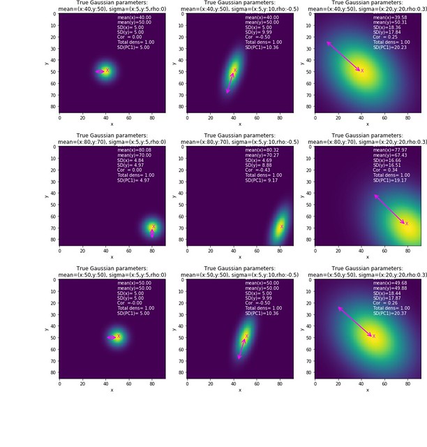
Plot the first PC component
Finally, plot the 1st PC
def plot_gaussian_kernel_with_exsimates(ms,sigmas,meanNN_TF=False,normalize_density=False):
    fig = plt.figure(figsize=(20,20))
    count = 1
    for (mx, my) in ms:
        for sigma in sigmas:
            # -----------------------
            # create a heatmap data
            arr = biv_gaussian_k(mx, my,
                                 sigma,
                                 width=width,
                                 height=height)
            const = biv_gaussian_constant(sigma)
            normalized_arr = const*arr

            # -----------------------
            # normalization Recommended!
            if normalize_density:
                normalized_arr /=np.sum(normalized_arr)
            #normalized_arr[normalized_arr < 0.000001 ] =0

            # ------------------------------
            # mean and variance estimation
            cov = get_cov(normalized_arr, meanNN_TF=meanNN_TF)
            sdx = get_merginal_sd(normalized_arr,dim="x", meanNN_TF=meanNN_TF)
            sdy = get_merginal_sd(normalized_arr,dim="y", meanNN_TF=meanNN_TF)
            r = cov/(sdx*sdy)
            meanx = get_merginal_mean(normalized_arr,dim="x", meanNN_TF=meanNN_TF)
            meany = get_merginal_mean(normalized_arr,dim="y", meanNN_TF=meanNN_TF)

            # -----------------------------
            # PCA
            est_sigma_mat = np.array([ [sdx**2, cov],
                                       [cov,    sdy**2]])

            evl, evec = fit_PCA(est_sigma_mat)
            SDPC1 = np.sqrt(evl[0])
            # ------------------------
            # plot
            ax = fig.add_subplot(len(ms),len(sigmas),count)
            ax.imshow(arr)
            ax.set_xlabel("x")
            ax.set_ylabel("y")
            ax.set_title("True Gaussian parameters:\nmean=(x:{},y:{}), sigma=(x:{},y:{},rho:{})".format(mx,my,*sigma))
            ax.text(meanx,meany,"X",color="magenta")
            ax.text(50,30,"Estimates:\nmean(x)={:5.2f}\nmean(y)={:5.2f}\nSD(x)={:5.2f}\nSD(y)={:5.2f}\nCor  ={:5.2f}\nTotal dens={:5.2f}\nSD(PC1)={:5.2f}".format(
                meanx,meany,sdx,sdy,r,np.sum(normalized_arr),SDPC1),color="white")
            count += 1

            # -----------------------
            # plot The 1st principal component
            ax.annotate("",
                fontsize=20,
                xytext = (meanx,meany),
                xy     = (meanx-2*SDPC1*evec[0,0],
                          meany-2*SDPC1*evec[1,0]),
                arrowprops = {"arrowstyle":"<->",
                              "color":"magenta",
                              "linewidth":2}
                )
    #plt.savefig("plot_PCA_from_heatmap.png",bbox_inches='tight',pad_inches=0)
    #plt.close()
    plt.show()


plot_gaussian_kernel_with_exsimates(ms,sigmas,meanNN_TF=True,normalize_density=True)
