My goal of this blog post is to understand Local Binary Pattern (LBP) texture operator. It is a simple yet very powerful algorithm to understand image. With the features created by the LBP texture operator, we can tell the texture of the objects in image; The features can, for example, separate images of carpet from image of blicks. That sounds very cool and I want to understand LBP texutre operator better.
Scholarpedia discribes LBP as:
Local Binary Pattern (LBP) is a simple yet very efficient texture operator which labels the pixels of an image by thresholding the neighborhood of each pixel and considers the result as a binary number.This sentence is very dense, and hard to understand if this is your first time learning the LBP. So I will implement every step of LBP calculation to understand what's exactly going on.
Reference
LBP texture operator
LBPs compute a local representation of texture. This local representation is constructed by comparing each pixel with its surrounding neighborhood of pixels.
In more details, the following is the LBP's calculation steps. (Please reference the Kelvin Salton do Prado's Toward Data Science blog's figure below.)
- Step 0: Convert an image to grayscale
- Step 1: 3 by 3 pixel: For each pixel in the grayscale image, we select a neighborhood of size r, say three, surrounding the center pixel.
- Step 2: Binary operation: For each pixel's three by three neighboor, compapre the center value and its neighboor values. If the neighboor values are greater than center, record 1 else record 0.
- Step 3: Decimal: Convert the binary operated values to a digit.
Step 3 needs more details. First, we the 8 surrounding neighboor pixels in clockwise or counter-clockwise. The starting pixel can be any of the 8 neighboor values as long as it is consistent.
Let LBP value to be 0 and then if the binary value of the starting pixel is one, add $2^0$ to the LBP value, else 0. If the next binary value is one, add $2^1$, else add 0. If the next binary value is one, add $2^2$, else add 0.
Repeat this process until the last pixel.
For example in the Kelvin Salton do Prado's graph below, setting topleft corner as the strting pixel, and ordering the neighboor pixel values in clock wise manner, we can convert the binary operated values to a digit as:
$$
141 = 2^0 + 2^2+2^3+2^7
$$
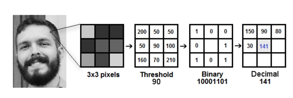 Image cited from Kelvin Salton do Prado's Toward Data Science blog
Now you understand how LBP algorithm works. Let's use it to real images. Here, I read in 8 images. The four of them is the image of blind in my window. And the remaining four are the images of my carpets. I took these pictures using my iphone. All the images have the same shape.
import matplotlib.pyplot as plt
import cv2, os
import numpy as np
dir_images = "LBPdata/"
imgs = os.listdir(dir_images)
fig = plt.figure(figsize=(20,14))
for count, imgnm in enumerate(imgs,1):
image = plt.imread(os.path.join(dir_images,imgnm))
ax = fig.add_subplot(2,len(imgs)/2,count)
ax.imshow(image)
ax.set_title(imgnm)
plt.show()

The following implement LBP calculation.
def getLBPimage(gray_image):
'''
== Input ==
gray_image : color image of shape (height, width)
== Output ==
imgLBP : LBP converted image of the same shape as Understand LBP histogram
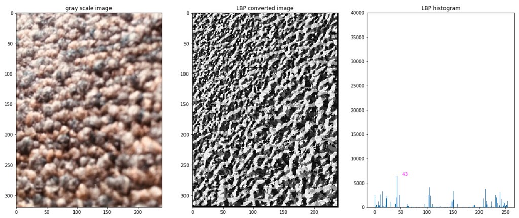
Notice that the histograms only range between 0 and $2^8 -1 = 255$, because there are only eight neighboor values for each pixel values. Clearly, we see the similar LBP histograms within the same image categories, and the LBP histograms are quite different across blinds and carpet.
Blinds
The histograms show peaks at 147, 149 and 221. These patterns corresponds to non-uniform regions. See diagram below:
|x x o|
|x c o|
|o o x|
LBP value = 2**0 + 2**1 + 2**4 + 2**7 = 147
diagram 3|x o x|
|x c o|
|o o x|
LBP value = 2**0 + 2**2 + 2**4 + 2**7 = 149
diagram 4|x x o|
|x c o|
|x o x|
LBP value = 2**0 + 2**1 + 2**4 + 2**6 + 2**7 = 211
diagram 5Carpet:
The histograms show peaks at small values (0) and largest values ($2^8$). These LBP values show that the regions are very flat.
|x x x|
|x c x|
|x x x|
LBP value = 0
diagram 1 (x: pixels that are less intense than c)|o o o|
|o c o|
|o o o|
LBP value = 2**0 + 2**1 + 2**2 + 2**3 + 2**4 + 2**5 + 2**6 + 2**7 = 255
diagram 2 (o: pixels that are more intense than c))dir_images = "LBPdata/"
imgs = os.listdir(dir_images)
for imgnm in imgs:
image = plt.imread(os.path.join(dir_images,imgnm))
imgLBP = getLBPimage(image)
vecimgLBP = imgLBP.flatten()
fig = plt.figure(figsize=(20,8))
ax = fig.add_subplot(1,3,1)
ax.imshow(image)
ax.set_title("gray scale image")
ax = fig.add_subplot(1,3,2)
ax.imshow(imgLBP,cmap="gray")
ax.set_title("LBP converted image")
ax = fig.add_subplot(1,3,3)
freq,lbp, _ = ax.hist(vecimgLBP,bins=2**8)
ax.set_ylim(0,40000)
lbp = lbp[:-1]
## print the LBP values when frequencies are high
largeTF = freq > 5000
for x, fr in zip(lbp[largeTF],freq[largeTF]):
ax.text(x,fr, "{:6.0f}".format(x),color="magenta")
ax.set_title("LBP histogram")
plt.show()


