In this blog post, we will generate adversarial images for a pre-trained Keras facial keypoint detection model.
What is adversarial images?
According to OpenAI, adversarial examples are:
inputs to machine learning models that an attacker has intentionally designed to cause the model to make a mistake; they’re like optical illusions for machines.
Explaining and Harnessing Adversarial Examples proposed the fast gradient sign method that generates an adversarial example as:
$$ X' = X + \epsilon sign \left(\frac{d \textrm{loss}(X)}{dX} \right) $$ where $\epsilon$ is a small value such that the max-norm of the perturbation is bounded.
This means that the adversarial perturbation creates a new training example by adding a perturbation along a direction which the network is likely to increase the loss. Explaining and Harnessing Adversarial Examples mentioned that by including the adversarial examples in the training data, the classifier becomes more robust. This is adversarial training.
Adversarial examples using TensorFlow
The goal of this blog is to understand and create adversarial examples using TensorFlow. I will use TensorFlow rather than Keras as writing it in Keras requires Keras's backend functions which essentially requires using Tensorflow backend functions. Rather than mixing up the two frameworks, I will stick to TensorFlow.
I will use my facial keypoint detection model developed using Kaggle's facial keypoint detection data as a base model for which I will create adversarial examples. See Achieving Top 23% in Kaggle's Facial Keypoints Detection with Keras + Tensorflow to learn how I developed this model.
As this model is developed in Keras, the first half of the blog discusses how to read in the Keras's pre-trained model, and load TensorFlow's model. If you already have a TensorFlow model in hand, I recommend you to start reading it from the section "Create a class for adversarial examples with TensorFlow deep learning model".
Reference
import matplotlib.pyplot as plt
import pandas as pd
import numpy as np
import tensorflow as tf
import os, sys


os.environ["CUDA_DEVICE_ORDER"] = "PCI_BUS_ID"
config = tf.ConfigProto()
config.gpu_options.per_process_gpu_memory_fraction = 0.95
config.gpu_options.visible_device_list = "1"
tf.Session(config=config)


print("python {}".format(sys.version))
print("tensorflow version {}".format(tf.__version__))

## change the directory
os.chdir("../FacialKeypoint/")
Read in a Keras's pre-trained model and save it as a TensorFlow model
This deep learning model takes input image of size (94,94,1) and output the standardized (x,y)-coordinates of the 15 landmark. That is, there are 30 targets to estimate (x-coordinate of left eye, y-coordinate of left eye, x-coordinate of nose,....). The model was developed at Achieving Top 23% in Kaggle's Facial Keypoints Detection with Keras + Tensorflow.
from keras.models import model_from_json

def load_model(name):
    model = model_from_json(open(name+'_architecture.json').read())
    model.load_weights(name + '_weights.h5')
    return(model)

model = load_model("model4")
model.summary()
Create a directory to save a TensorFlow model.
outdir = "model4_tf"
try:
    os.mkdir(outdir )
except:
    pass
The codes in the next block are mostly based on amir-abdi's Github code.
# Write the graph in binary .pb file
from tensorflow.python.framework import graph_util
from tensorflow.python.framework import graph_io
from keras import backend as K

prefix = "simple_cnn"
name = 'output_graph.pb'
# Alias the outputs in the model - this sometimes makes them easier to access in TF
pred = []
pred_node_names = []
for i, o in enumerate(model.outputs):
        pred_node_names.append(prefix+'_'+str(i))
        pred.append(tf.identity(o,
                                name=pred_node_names[i]))
print('Output nodes names are: ', pred_node_names)


sess = K.get_session()

# Write the graph in human readable
# f = 'graph_def_for_reference.pb.ascii'
# tf.train.write_graph(sess.graph.as_graph_def(), outdir, f, as_text=True)
# print('Saved the graph definition in ascii format at: ',  os.path.join(outdir, f))

constant_graph = graph_util.convert_variables_to_constants(sess,
                                                           sess.graph.as_graph_def(),
                                                           pred_node_names)
graph_io.write_graph(constant_graph, outdir, name, as_text=False)
## Finally delete the Keras's session
K.clear_session()
outdir = "../FacialKeypoint/model4_tf"
name = 'output_graph.pb'

## Make sure that there are no defult graph

tf.reset_default_graph()

def load_graph(model_name):
    #graph = tf.Graph()
    graph = tf.get_default_graph()
    graph_def = tf.GraphDef()
    with open(model_name, "rb") as f:
        graph_def.ParseFromString(f.read())
    with graph.as_default():
        tf.import_graph_def(graph_def)
    return graph
my_graph = load_graph(model_name=os.path.join(outdir, name))
In order to generate adversarial examples, I need to calculate the gradient of loss with respect to the image as: $$ \frac{d \textrm{loss}(y,X)}{dX} $$ where my loss function for the landmark detection model was MSE: $$ \textrm{loss}(y,X) = (y - f(X))^2 $$
For the gradient calculation, I need a input tensor (import/conv2d_22_input) and output tensor (import/simple_cnn_0) The following codes show all the operations' names in the Tensor's graph. We can find the tensors that we need:
- $f(X)$ = import/simple_cnn_0
- $X$ = import/conv2d_22_input
for i, op in enumerate(tf.get_default_graph().get_operations()):
    print "{: 3.0f}: {}".format(i,op.name)
Extract only tensors that are needed for calculating the gradients:
input_op = my_graph.get_operation_by_name("import/conv2d_22_input")
output_op = my_graph.get_operation_by_name("import/simple_cnn_0")
ops = (input_op,output_op)
Following class computes the adversarial examples for given value of $\epsilon$, image $X$ and true landmark coordinate vector $y$.
class AdversarialImage(object):
    def __init__(self,inp,out,eps=0.01):
        '''
        inp : input tensor  (image)
        out : output tensor (y_pred)
        eps : scalar
        '''
        self.inp = inp.outputs[0]
        self.out = out.outputs[0]
        self.define_aimage_tensor(float(eps))

    def mse_tf(self,y_pred,y_test, verbose=True):
        '''
        y_pred : tensor
        y_test : tensor having the same shape as y_pred
        '''
        ## element wise square
        minus  = tf.constant(-1.0)
        m_y_test = tf.scalar_mul(minus,y_test)
        square = tf.square(tf.add(y_pred ,m_y_test))## preserve the same shape as y_pred.shape
        ## mean across the final dimensions
        ms = tf.reduce_mean(square)
        return(ms)

    def define_aimage_tensor(self,eps):
        '''
        Define a graph to output adversarial image

        Xnew = X + eps * sign(dX)

        X : np.array of image of shape (None,height, width,n_channel)
        y : np.array containing the true landmark coordinates (None, 30)
        '''
        ## get list of target
        yshape = [None] + [int(i) for i in self.out.get_shape()[1:]]
        eps_tf = tf.constant(eps,name="epsilon")

        y_true_tf = tf.placeholder(tf.float32, yshape)
        y_pred_tf = self.out

        loss = self.mse_tf(y_pred_tf,y_true_tf)

        ## tensor that calculate the gradient of loss with respect to image i.e., dX
        grad_tf          = tf.gradients(loss,[self.inp])
        grad_sign_tf     = tf.sign(grad_tf)
        grad_sign_eps_tf = tf.scalar_mul(eps_tf,
                                         grad_sign_tf)
        new_image_tf = tf.add(grad_sign_eps_tf,self.inp)

        self.y_true  = y_true_tf
        self.eps     = eps_tf
        self.aimage  = new_image_tf
        self.added_noise = grad_sign_eps_tf


    def predict(self,X):

        with tf.Session() as sess:
            y_pred = sess.run(self.out,
                              feed_dict={self.inp:X})
        return(y_pred)
    def get_aimage(self,X,y,added_noise=False):
        tensor2eval = [self.aimage]
        if added_noise:
            tensor2eval.append(self.added_noise)

        with tf.Session() as sess:
            result = sess.run(tensor2eval,
                              feed_dict={self.inp:X,
                                         self.y_true:y
                                         })
        for i in range(len(result)):
            result[i] = result[i].reshape(*X.shape)
        return(result)
Load Kaggle's facial landmark detection data
Finally, let's generate the adversarial examples using Kaggle's facial landmark detection data. The data extraction and transformation process is the same as my previous blogs:
- Achieving Top 23% in Kaggle's Facial Keypoints Detection with Keras + Tensorflow
- Achieving top 5 in Kaggle's facial keypoints detection using FCN.
I will use the same ETL functions as before.
def plot_sample(X,y,axs):
    '''
    kaggle picture is 96 by 96
    y is rescaled to range between -1 and 1
    '''

    axs.imshow(X.reshape(96,96),cmap="gray")
    axs.scatter(48*y[0::2]+ 48,48*y[1::2]+ 48)

def load(test=False, cols=None):
    """
    load test/train data
    cols : a list containing landmark label names.
           If this is specified, only the subset of the landmark labels are
           extracted. for example, cols could be:

          [left_eye_center_x, left_eye_center_y]

    return:
    X: 2-d numpy array (Nsample, Ncol*Nrow)
    y: 2-d numpy array (Nsample, Nlandmarks*2)
       In total there are 15 landmarks.
       As x and y coordinates are recorded, u.shape = (Nsample,30)

    """
    from pandas import read_csv
    from sklearn.utils import shuffle

    fname = FTEST if test else FTRAIN
    df = read_csv(os.path.expanduser(fname))


    df['Image'] = df['Image'].apply(lambda im: np.fromstring(im, sep=' '))

    if cols:
        df = df[list(cols) + ['Image']]

    myprint = df.count()
    myprint = myprint.reset_index()
    print(myprint)
    ## row with at least one NA columns are removed!
    df = df.dropna()


    X = np.vstack(df['Image'].values) / 255.  # changes valeus between 0 and 1
    X = X.astype(np.float32)

    if not test:  # labels only exists for the training data
        ## standardization of the response
        y = df[df.columns[:-1]].values
        y = (y - 48) / 48  # y values are between [-1,1]
        X, y = shuffle(X, y, random_state=42)  # shuffle data
        y = y.astype(np.float32)
    else:
        y = None


    return X, y

def load2d(test=False,cols=None):

    re = load(test, cols)

    X = re[0].reshape(-1,96,96,1)
    y = re[1]

    return X, y

FTRAIN = 'data/training.csv'
FTEST = 'data/test.csv'
FIdLookup = 'data/IdLookupTable.csv'
X, y = load2d(test=False)
Let's instantiate two Adversarial Image class objects with two different values of epsilon. Notice that I instantiated the objects with positive and negative epsilon values. By changing the direction of sign to negative I can create "good" or "friendly" or "anti-adversarial" examples that can decrease the loss.
AIbad  = AdversarialImage(*ops,eps=0.01)
AIgood = AdversarialImage(*ops,eps=-0.01)
Generate adversarial images as well as good images, and visualize them together with RMSE.
Adversarial images increase the RMSE while "good" images decreases the RMSE. However, these images look identical to the original image to me!
def getrmse(y_pred,y_true):
    return(np.sqrt(np.mean((y_pred - y_true)**2)))
def getRMSE(y_pred,y_true):
    return("RMSE:{:4.3f}".format(getrmse(y_pred,y_true)))

Nplot = 5
inds = np.random.choice(X.shape[0],Nplot,replace=False)

count = 1
plt.close()
fig = plt.figure(figsize=(20,20))
for irow in inds:
    Xi, yi = X[[irow]], y[[irow]]
    ## original image
    y_predi              = AIgood.predict(Xi)

    ## Good image
    (X_good, noise_good) = AIgood.get_aimage(Xi,yi,added_noise=True)
    y_predi_good          = AIgood.predict(X_good)

    ## Adversarial image
    (X_bad, noise_bad)   = AIbad.get_aimage(Xi,yi,added_noise=True)
    y_predi_bad          = AIbad.predict(X_bad)

    ## ======== ##
    ## Plotting
    ## ======== ##

    ## original image
    axs = fig.add_subplot(Nplot,5,count)
    plot_sample(Xi[0],y_predi[0],axs)
    axs.set_title("original" + getRMSE(y_predi,yi))
    count += 1

    ## noise for bad image
    axs = fig.add_subplot(Nplot,5,count)
    axs.imshow(noise_bad.reshape(96,96),cmap="gray")
    axs.set_title("Noise for adversarial image")
    count += 1

    ## bad image
    axs = fig.add_subplot(Nplot,5,count)
    plot_sample(X_bad[0],y_predi_bad[0],axs)
    axs.set_title("Adversarial image: " + getRMSE(y_predi_bad,yi))
    count += 1

    ## noise for good image
    axs = fig.add_subplot(Nplot,5,count)
    axs.imshow(noise_good.reshape(96,96),cmap="gray")
    axs.set_title("Noise for good image")
    count += 1

    ## good image
    axs = fig.add_subplot(Nplot,5,count)
    plot_sample(X_good[0],y_predi_good[0],axs)
    axs.set_title("Good image: " + getRMSE(y_predi_good,yi))
    count += 1

plt.show()

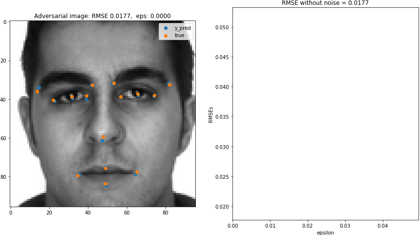
Think about the effect of $\epsilon$ on adversarial images
To create adversarial example, it is very important to choose "good" value of $\epsilon$, that determines the amount of noise added to the original image $X$. The maginitude of $\epsilon$ should depend on the range of X. Our pixcel values in X ranges from 0 to 1 after standardization. See histogram below.
vecX = X.flatten()
plt.hist(vecX[~np.isnan(vecX)])
plt.xlabel("X")
plt.show()

Simple and Scalable Predictive Uncertainty Estimation using Deep Ensembles previously give recommendation to the default values of $\epsilon$ in his adversarial training.
Recommended default values are... $\epsilon = 1\%$ of input range of the corresponding dimension (e.g. 2.55 if input range is [0,255]).
Therefore in our data, it would be interesting to see the effect of $\epsilon$ around the values of 0.01.
Let's create gif that shows the effect of $\epsilon$ on adversarial image and the RMSE. This will be the gif shown at the beggining of the blog.
dir_images = "adversarial_image_gif/"
try:
    os.mkdir(dir_images)
except:
    pass
irow = 1072
Xi, yi = X[[irow]], y[[irow]]
## original image
y_predi              = AIbad.predict(Xi)

rmse_base = getrmse(y_predi,yi)

## range of epsilon
xs = np.arange(0,0.05,0.0005)

rmses = np.array([np.NaN]*len(xs))
for ieps, eps in enumerate(xs):


    AIbad  = AdversarialImage(*ops,eps=eps)

    ## Adversarial image
    (X_bad, noise_bad)   = AIbad.get_aimage(Xi,yi,added_noise=True)
    y_predi_bad          = AIbad.predict(X_bad)

    ## ======== ##
    ## Plotting
    ## ======== ##
    count = 1

    fig = plt.figure(figsize=(15,8))


    ## noise for bad image
    rmses[ieps] = getrmse(y_predi_bad,yi)
    axs = fig.add_subplot(1,2,count)
    axs.imshow(X_bad[0].reshape(96,96),cmap="gray")
    axs.scatter(48*y_predi_bad[0][0::2]+ 48,
                48*y_predi_bad[0][1::2]+ 48,label="y_pred")
    axs.scatter(48*yi[0][0::2]+ 48,
                48*yi[0][1::2]+ 48,label="true")
    axs.set_title("Adversarial image: RMSE {:5.4f},  eps: {:5.4f}".format(rmses[ieps],eps))
    plt.legend()
    count += 1

    ## noise for bad image
    axs = fig.add_subplot(1,2,count)
    axs.plot(xs,rmses)
    axs.set_xlim([np.min(xs),np.max(xs)])
    axs.set_ylim([rmse_base,rmse_base*3])
    axs.set_ylabel("RMSEs")
    axs.set_xlabel("epsilon")
    axs.set_title("RMSE without noise = {:5.4f}".format(rmses[0]))
    count += 1

    plt.savefig( dir_images + '/{:05.0f}.png'.format(ieps),bbox_inches='tight',pad_inches=0)
Create a gif presented at the beginning of this blog
def makegif(dir_images):
    import imageio
    filenames = np.sort(os.listdir(dir_images))
    filenames = [ fnm for fnm in filenames if ".png" in fnm]

    with imageio.get_writer(dir_images + '/image.gif', mode='I') as writer:
        for filename in filenames:
            image = imageio.imread(dir_images + filename)
            writer.append_data(image)
            os.remove(dir_images + filename)

makegif(dir_images)