This is the first blog post of "Object Detection with R-CNN" series.
Object detection
According to the wikipedia:
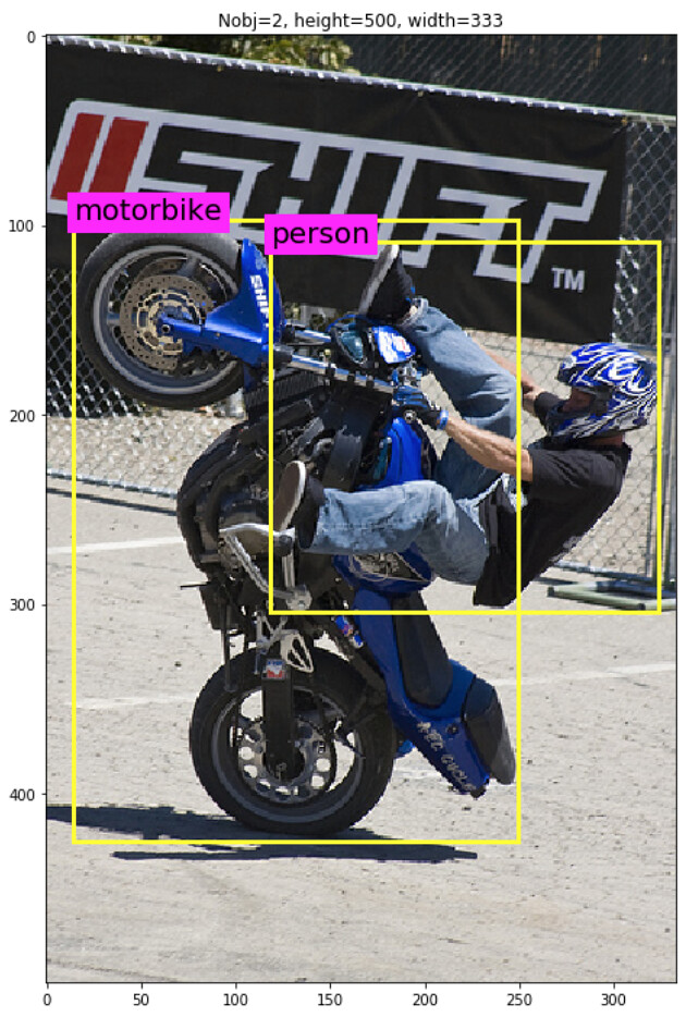
Object detection is a computer technology related to computer vision and image processing that deals with detecting instances of semantic objects of a certain class (such as humans, buildings, or cars) in digital images and videos.In the image above, you see a mortor cyclist and If you follow all the blog posts in this series, you are able to understand every step of the R-CNN. All the blog posts use PASCAL VOC 2012 data as an example.
Visual Object Classes Challenge 2012 (VOC2012)
The main goal of visual object classes challenge 2012 (VOC2012) is to recognize objects from a number of visual object classes in realistic scenes. It is a supervised learning learning problem in that a training set of labelled images is provided.
The twenty object classes that have been selected are:
- Person: person
- Animal: bird, cat, cow, dog, horse, sheep
- Vehicle: aeroplane, bicycle, boat, bus, car, motorbike, train
- Indoor: bottle, chair, dining table, potted plant, sofa, tv/monitor
The main competition tasks that I discuss in this blog series are the detection of objects (where it the object? can you create a rectangle bounding box around the object?) and the classification of objects (is this object a person or a cat?).

What is the goals of this blog?
This first blog post of the series has three goals:
- Section 1: Set up the computing environments by setting up python.
- Section 2: Prepare PASCAL VOC2012 data
- Section 3: Understand PASCAL VOC2012 data and preprocess data.
Let's get started!
Reference: "Object Detection with R-CNN" series in my blog
Reference: "Object Detection with R-CNN" series in my Github
Section 1: Setup environments
I am using Mac OS and I recommend readers to use Mac or Linux environment. (Sorry for Windows users).
To follow the blog series, please install the followings:
Anaconda 3.7
Please visit Anaconda 3.7 for installation.

Keras and Tensorflow
In the later blog Part 4: Object detection with Pascal data - CNN feature extraction, you will also need Keras and tensorflow installed in your environment. These are very popular deep learning frameworks. You do NOT need GPU to follow this blog series as we will only use pre-trained network. To install them, from your terminal run the following codes:
pip install tensorflow
pip install keras
Section 2: Prepare PASCAL VOC2012 data
Step 1: Download PASCAL VOC2012 data
Data can be downloaded by visiting Visual Object Classes Challenge 2012 (VOC2012), and click Download the training/validation data (2GB tar file). Choose the location to download the data to be the current working directory of this ipython notebook. Downloading the data took me roughtly 6 minutes in my local computer.

Step 2: Untar the downloaded folder
Untar the downloaded folder "VOCtrainval_11-May-2012.tar". Now your current working directory should look something like this:

Record the relative path to the Annotations folder and JPEG image folder.
dir_anno = "VOCdevkit/VOC2012/Annotations"
img_dir = "VOCdevkit/VOC2012/JPEGImages"
Let's look at the downloaded data using linux command. Following commands first count the number of files in Annotations folder and the first 10 file names.
ls $dir_anno | wc -l; ls $dir_anno | head -10
Run the same command for the JPEGImages data. In total, there are 17125 xml files in Annotations folder and 17125 jpeg files in JPEGImages folder.
ls $img_dir | wc -l;ls $img_dir | head -10
Section 3: Understand PASCAL VOC2012 data and preprocess data
Understand annotation data
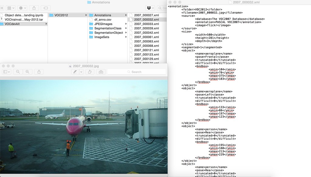
For each image jpg file in JPEGImages folder, there is corresponding .xml file in Annotation folder. Let's take a look at one of the xml file (2007_00032.xml) and its corresponding image (2007_00032.jpg).
The image contains 2 airplanes and 2 people. So there are 4 objects in total. The bounding box of these four objects are recorded in xml file as follow.

Having annotation infomation of each image in separate file is a bit hard to work with. We first aggregate all these xml files into a single csv file using panda modules.
Here we will first create a panda dataframe "df_anno" containing annotations, and then save it into a csv file.
- each row of df_anno corresponds to a single frame.
- df_anno contains 285 columns.
- width: width of the frame
- height: height of the frame
- Nobj : The number of objects in the frame
- fileID: The png file name
- For each frame, there are at most 56 objects in one frame. The infomation of the ith object is recorded in df_anno as:
bbx_i_nm: The type of object inside of the bounding box i e.g.,bbx_i_xmin: The x coordinate of the minimum corner in bounding box ibbx_i_ymin: The y coordinate of the minimum corner in bounding box ibbx_i_xmax: The x coordinate of the maximum corner in bounding box ibbx_i_ymax: The y coordinate of the maximum corner in bounding box i
import os
import numpy as np
import xml.etree.ElementTree as ET
from collections import OrderedDict
import matplotlib.pyplot as plt
import pandas as pd
def extract_single_xml_file(tree):
Nobj = 0
row = OrderedDict()
for elems in tree.iter():
if elems.tag == "size":
for elem in elems:
row[elem.tag] = int(elem.text)
if elems.tag == "object":
for elem in elems:
if elem.tag == "name":
row["bbx_{}_{}".format(Nobj,elem.tag)] = str(elem.text)
if elem.tag == "bndbox":
for k in elem:
row["bbx_{}_{}".format(Nobj,k.tag)] = float(k.text)
Nobj += 1
row["Nobj"] = Nobj
return(row)
df_anno = []
for fnm in os.listdir(dir_anno):
if not fnm.startswith('.'): ## do not include hidden folders/files
tree = ET.parse(os.path.join(dir_anno,fnm))
row = extract_single_xml_file(tree)
row["fileID"] = fnm.split(".")[0]
df_anno.append(row)
df_anno = pd.DataFrame(df_anno)
maxNobj = np.max(df_anno["Nobj"])
print("columns in df_anno\n-----------------")
for icol, colnm in enumerate(df_anno.columns):
print("{:3.0f}: {}".format(icol,colnm))
print("-"*30)
print("df_anno.shape={}=(N frames, N columns)".format(df_anno.shape))
df_anno.head()
Save df_anno as a csv file in the current folder
# location to save df_anno.csv
dir_preprocessed = "VOCdevkit/VOC2012"
df_anno.to_csv(os.path.join(dir_preprocessed,"df_anno.csv"),index=False)
Now you should see df_anno.csv file in the directory VOCdevkit/VOC2012.

plt.hist(df_anno["Nobj"].values,bins=100)
plt.title("max N of objects per image={}".format(maxNobj))
plt.show()
Count the number of objects in each class for each object type
- In total 20 object types exist.
- Bar plot shows that "person" class is by far the largest and there are 17401 "person" objects in the entire data.
from collections import Counter
class_obj = []
for ibbx in range(maxNobj):
class_obj.extend(df_anno["bbx_{}_name".format(ibbx)].values)
class_obj = np.array(class_obj)
count = Counter(class_obj[class_obj != 'nan'])
print(count)
class_nm = list(count.keys())
class_count = list(count.values())
asort_class_count = np.argsort(class_count)
class_nm = np.array(class_nm)[asort_class_count]
class_count = np.array(class_count)[asort_class_count]
xs = range(len(class_count))
plt.barh(xs,class_count)
plt.yticks(xs,class_nm)
plt.title("The number of objects per class: {} objects in total".format(len(count)))
plt.show()
import imageio
def plt_rectangle(plt,label,x1,y1,x2,y2):
'''
== Input ==
plt : matplotlib.pyplot object
label : string containing the object class name
x1 : top left corner x coordinate
y1 : top left corner y coordinate
x2 : bottom right corner x coordinate
y2 : bottom right corner y coordinate
'''
linewidth = 3
color = "yellow"
plt.text(x1,y1,label,fontsize=20,backgroundcolor="magenta")
plt.plot([x1,x1],[y1,y2], linewidth=linewidth,color=color)
plt.plot([x2,x2],[y1,y2], linewidth=linewidth,color=color)
plt.plot([x1,x2],[y1,y1], linewidth=linewidth,color=color)
plt.plot([x1,x2],[y2,y2], linewidth=linewidth,color=color)
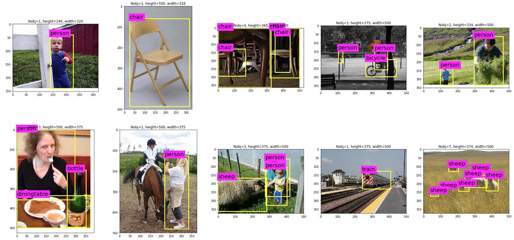
# randomly select 20 frames
size = 20
ind_random = np.random.randint(0,df_anno.shape[0],size=size)
for irow in ind_random:
row = df_anno.iloc[irow,:]
path = os.path.join(img_dir, row["fileID"] + ".jpg")
# read in image
img = imageio.imread(path)
plt.figure(figsize=(12,12))
plt.imshow(img) # plot image
plt.title("Nobj={}, height={}, width={}".format(row["Nobj"],row["height"],row["width"]))
# for each object in the image, plot the bounding box
for iplot in range(row["Nobj"]):
plt_rectangle(plt,
label = row["bbx_{}_name".format(iplot)],
x1=row["bbx_{}_xmin".format(iplot)],
y1=row["bbx_{}_ymin".format(iplot)],
x2=row["bbx_{}_xmax".format(iplot)],
y2=row["bbx_{}_ymax".format(iplot)])
plt.show() ## show the plot